Check for heteroskedasticity in OLS with lmtest package in R

One core assumption when calculating ordinary least squares regressions is that all the random variables in the model have equal variance around the best fitting line.

Essentially, when we run an OLS, we expect that the error terms have no fan pattern.

Example of homoskedasticiy

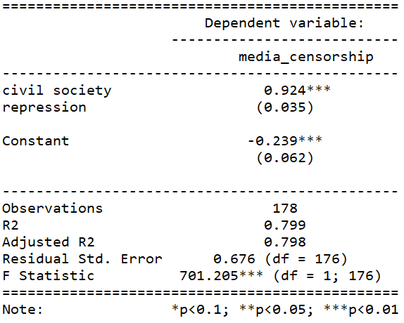
So let’s look at an example of this assumption being satisfied. I run a simple regression to see whether there is a relationship between and media censorship and civil society repression in 178 countries in 2010.

ggplot(data_010, aes(media_censorship, civil_society_repression)) 
      + geom_point() + geom_smooth(method = "lm") 
      + geom_text(size = 3, nudge_y = 0.1, aes(label = country))

If we run a simple regression

summary(repression_model <- lm(media_censorship ~ civil_society_repression, data = data_2010))
stargazer(repression_model, type = "text")

This is pretty common sense; a country that represses its citizens in one sphere is more likely to repress in other areas. In this case repressing the media correlates with repressing civil society.

We can plot the residuals of the above model with the autoplot() function from the ggfortify package.

library(ggfortify)
autoplot(repression_model)

Nothing unusual appears to jump out at us with regard to evidence for heteroskedasticity!

In the first Residuals vs Fitted plot, we can see that blue line does not drastically diverge from the dotted line (which indicates residual value = 0).

The third plot Scale-Location shows again that there is no drastic instances of heteroskedasticity. We want to see the blue line relatively horizontal. There is no clear pattern in the distribution of the residual points.

In the Residual vs. Leverage plot (plot number 4), the high leverage observation 19257 is North Korea! A usual suspect when we examine model outliers.

While it is helpful to visually see the residuals plotted out, a more objective test can help us find whether the model is indeed free from heteroskedasticity problems.

For this we need the Breusch-Pagan test for heteroskedasticity from the lmtest package.

install.packages("lmtest)
library(lmtest)
bptest(repression_model)

The default in R is the studentized Breusch-Pagan. However if you add the studentize = FALSE argument, you have the non-studentized version

The null hypothesis of the Breusch-Pagan test is that the variance in the model is homoskedastic.

With our repression_model, we cannot reject the null, so we can say with confidence that there is no major heteroskedasticity issue in our model.

The non-studentized Breusch-Pagan test makes a very big assumption that the error term is from Gaussian distribution. Since this assumption is usually hard to verify, the default bptest() in R “studentizes” the test statistic and provide asymptotically correct significance levels for distributions for error.

Why do we care about heteroskedasticity?

If our model demonstrates high level of heteroskedasticity (i.e. the random variables have non-random variation across observations), we run into problems.

Why?

• OLS uses sub-optimal estimators based on incorrect assumptions and

• The standard errors computed using these flawed least square estimators are more likely to be under-valued. Since standard errors are necessary to compute our t – statistics and arrive at our p – value, these inaccurate standard errors are a problem.

Example of heteroskedasticity

Let’s look at an example of this homoskedasticity assumption NOT being satisfied.

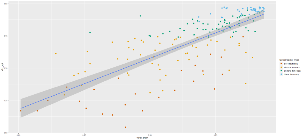
I run a simple regression to see whether there is a relationship between democracy score and respect for individuals’ private property rights in 178 countries in 2010.

When you are examining democracy as the main dependent variable, heteroskedasticity is a common complaint. This is because all highly democratic countries are all usually quite similar. However, when we look at autocracies, they are all quite different and seem to march to the beat of their own despotic drum. We cannot assume that the random variance across different regime types is equally likely.

First, let’s have a look at the relationship.

prop_graph <- ggplot(vdem2010, aes(v2xcl_prpty, v2x_api)) 
                     + geom_point(size = 3, aes(color = factor(regime_type))) 
                     + geom_smooth(method = "lm")
prop_graph + scale_colour_manual(values = c("#D55E00", "#E69F00", "#009E73", "#56B4E9"))

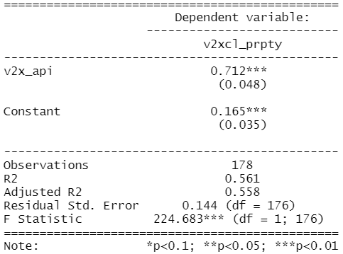
Next, let’s fit the model to examine the relationship.

summary(property_model <- lm(property_score ~ democracy_score, data = data_2010))
stargazer(property_model, type = "text")

To plot the residuals (and other diagnostic graphs) of the model, we can use the autoplot() function to look at the relationship in the model graphically.

autoplot(property_model)

Graph number 1 plots the residuals against the fitted model and we can see that lower values on the x – axis (fitted values) correspond with greater spread on the y – axis. Lower democracy scores relate to greater error on property rights index scores. Plus the blue line does not lie horizontal and near the dotted line. It appears we have non-random error patterns.

Examining the Scale – Location graph (number 3), we can see that the graph is not horizontal.

Again, interpreting the graph can be an imprecise art. So a more objective approach may be to run the bptest().

bptest(property_model)

Since the p – value is far smaller than 0.05, we can reject the null of homoskedasticity.

Rather, we have evidence that our model suffers from heteroskedasticity. The standard errors in the regression appear smaller than they actually are in reality. This inflates our t – statistic and we cannot trust our p – value.

In the next blog post, we can look at ways to rectify this violation of homoskedasticity and to ensure that our regression output has more accurate standard errors and therefore more accurate p – values.

Click here to use the sandwich package to fix heteroskedasticity in the OLS regression.