Click here to read PART ONE of the blog series on creating the Regional Economic Communities dataset

How to create a Regional Economic Communities dataset. PART ONE: Scraping data with rvest in R

Packages we will need:

library(tidyverse)
library(countrycode)
library(WDI)

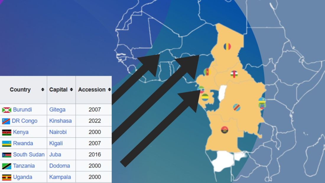
There are eight RECs in Africa. Some countries are only in one of the RECs, some are in many. Kenya is the winner with membership in four RECs: CEN-SAD, COMESA, EAC and IGAD.

In this blog, we will create a consolidated dataset for all 54 countries in Africa that are in a REC (or TWO or THREE or FOUR groups). Instead of a string variable for each group, we will create eight dummy group variables for each country.

To do this, we first make a vector of all the eight RECs.

patterns <- c("amu", "cen-sad", "comesa", "eac", "eccas", "ecowas", "igad", "sadc")

We put the vector of patterns in a for-loop to create a new binary variable column for each REC group.

We use the str_detect(rec_abbrev, pattern)) to see if the rec_abbrev column MATCHES the one of the above strings in the patterns vector.

The new variable will equal 1 if the variable string matches the pattern in the vector. Otherwise it will be equal to 0.

The double exclamation marks (!!) are used for unquoting, allowing the value of var_name to be treated as a variable name rather than a character string.

Then, we are able to create a variable name that were fed in from the vector dynamically into the for-loop. We can automatically do this for each REC group.

In this case, the iterated !!var_name will be replaced with the value stored in the var_name (AMU, CEN-SAD etc).

We can use the := to assign a new variable to the data frame.

The symbol := is called the “walrus operator” and we use it make or change variables without using quotation marks.

for (pattern in patterns) {
  var_name <- paste0(pattern, "_binary")
  rec <- rec %>%
    mutate(!!var_name := as.integer(str_detect(rec_abbrev, pattern)))
}

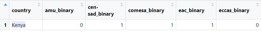
This is the dataset now with a binary variables indicating whether or not a country is in any one of the REC groups.

However, we quickly see the headache.

We do not want four rows for Kenya in the dataset. Rather, we only want one entry for each country and a 1 or a 0 for each REC.

We use the following summarise() function to consolidate one row per country.

rec %>%
group_by(country) %>%
  summarise(
    geo = first(geo),
    rec_abbrev = paste(rec_abbrev, collapse = ", "),
    across(ends_with("_binary"), ~ as.integer(any(. == 1)))) ->  rec_consolidated

The first() function extracts the first value in the geo variable for each country. This first() function is typically used with group_by() and summarise() to get the value from the first row of each group.

We use the the across() function to select all columns in the dataset that end with "_binary".

The ~ as.integer(any(. == 1)) checks if there’s any value equal to 1 within the binary variables. If they have a value of 1, the summarised data for each country will be 1; otherwise, it will be 0.

The following code can summarise each filtered group and add them to a new dataset that we can graph:

summ_group_pop <- function(my_df, filter_var, rec_name) {
  my_df %>%
    filter({{ filter_var }} == 1) %>% 
    summarize(total_population = sum(pop, na.rm = TRUE)) %>% 
    mutate(group = rec_name)
}

filter_vars <- c("amu_binary", "cen.sad_binary", "comesa_binary", 
                 "eac_binary", "eccas_binary", "ecowas_binary",
                 "igad_binary", "sadc_binary")
group_names <- c("AMU", "CEN-SAD", "COMESA", "EAC", "ECCAS", "ECOWAS",
                 "IGAD", "SADC")

rec_pop_summary <- data.frame()

for (i in seq_along(filter_vars)) {
  summary_df <- summ_group_pop(rec_wdi, !!as.name(filter_vars[i]), group_names[i])
  rec_pop_summary <- bind_rows(rec_pop_summary, summary_df)
}

And we graph it with geom_bar()

rec_pop_summary %>% 
  ggplot(aes(x = reorder(group, total_population),
             y = total_population)) + 
  geom_bar(stat = "identity", 
           width = 0.7, 
           color = "#0a85e5", 
           fill = "#0a85e5") +
  bbplot::bbc_style() + 
  scale_y_continuous(labels = scales::comma_format()) +
  coord_flip() + 
  labs(x = "RECs", 
       y = "Population", 
       title = "Population of REC groups in Africa", 
       subtitle = "Source: World Bank, 2022")

Cline Center Coup d’État Project Dataset

tailwind_palette <- c("001219","005f73","0a9396","94d2bd","e9d8a6","ee9b00","ca6702","bb3e03","ae2012","9b2226")

add_hashtag <- function(my_vec){
    hash_vec <-  paste0('#', my_vec)
    return(hash_vec)
  
  tailwind_hash <- add_hashtag(tailwind_palette)

Coups per million people in each REC

create_stateyears(system = "cow") %>% 
    add_democracy() -> demo

rec_wdi %>% 
  select(!c(year, country)) %>% 
  left_join(demo, by = c("cown" = "ccode")) %>% 
  filter(year > 1989) %>% 
  filter(amu_binary == 1) %>% 
  group_by(year) %>% 
  summarize(mean_demo = mean(v2x_polyarchy, na.rm = TRUE)) %>% 
  mutate(rec = "AMU") -> demo_amu

We can use a function to repeat the above code with all eight REC groups:

 create_demo_summary <- function(my_df, filter_var, group_name) {
  my_df %>%
    select(!c(year, country)) %>% 
    left_join(demo, by = c("cown" = "ccode")) %>% 
    filter(year > 1989) %>% 
    filter({{ filter_var }} == 1) %>% 
    group_by(year) %>% 
    summarize(mean_demo = mean(v2x_polyarchy, na.rm = TRUE)) %>% 
    mutate(rec = group_name)
}

rec_democracy_df <- data.frame()

for (i in seq_along(filter_vars)) {
  summary_df <- create_demo_summary(rec_wdi, !!as.name(filter_vars[i]), group_names[i])
  rec_democracy_df <- bind_rows(rec_democracy_df, summary_df)
}

And we graph out the average democracy scores cross the years

rec_democracy_df %>% 
  ggplot(aes(x = year, y = mean_demo, group = rec)) + 
  geom_line(aes(fill = rec, color = rec), size = 2, alpha = 0.8) + 
  # geom_point(aes(fill = rec, color = rec), size = 4) + 
  geom_label(data = . %>% group_by(rec) %>% filter(year == 2019), 
             aes(label = rec, 
                 fill = rec, 
                 x = 2019), color = "white",
             legend = FALSE, size = 3) +  
  scale_color_manual(values = tailwind_hash) + 
  scale_fill_manual(values = tailwind_hash) + 
  theme(legend.position = "none")