Packages we will need:
library(tidyverse)
library(haven)    # to read in the .sav file
library(magrittr)
In this blog, we will look at some ways to analyse survey data in R.
The data we will use is from the Afrobarometer survey.
This series examines and tracks public attitudes towards democracy, economic markets, and civil society in around 30 countries across the African continent.
Follow this link to download the latest round of data (round 8 from 2022).
https://www.afrobarometer.org/data/merged-data/
First we read in the SPSS .sav file:
ab <- read_sav(file.choose())The following code removes all the .sav metadata. This is so we can more easily play with it in R without it freaking out a bit.
ab[] <- lapply(ab, function(x) {attributes(x) <- NULL; x}) %>%
  as_tibble()
Next, we need to manually add the country_name variables.
ab %<>%
  mutate(country_name = case_when(
    COUNTRY == 2 ~ "Angola",
    COUNTRY == 3 ~ "Benin",
    COUNTRY == 4 ~ "Botswana",
    COUNTRY == 5 ~ "Burkina Faso",
    COUNTRY == 6 ~ "Cabo Verde",
    COUNTRY == 7 ~ "Cameroon",
    COUNTRY == 8 ~ "Côte d'Ivoire",
    COUNTRY == 9 ~ "Eswatini",
    COUNTRY == 10 ~ "Ethiopia",
    COUNTRY == 11 ~ "Gabon",
    COUNTRY == 12 ~ "Gambia",
    COUNTRY == 13 ~ "Ghana",
    COUNTRY == 14 ~ "Guinea",
    COUNTRY == 15 ~ "Kenya",
    COUNTRY == 16 ~ "Lesotho",
    COUNTRY == 17 ~ "Liberia",
    COUNTRY == 19 ~ "Malawi",
    COUNTRY == 20 ~ "Mali",
    COUNTRY == 21 ~ "Mauritius",
    COUNTRY == 22 ~ "Morocco",
    COUNTRY == 23 ~ "Mozambique",
    COUNTRY == 24 ~ "Namibia",
    COUNTRY == 25 ~ "Niger",
    COUNTRY == 26 ~ "Nigeria",
    COUNTRY == 28 ~ "Senegal",
    COUNTRY == 29 ~ "Sierra Leone",
    COUNTRY == 30 ~ "South Africa",
    COUNTRY == 31 ~ "Sudan",
    COUNTRY == 32 ~ "Tanzania",
    COUNTRY == 33 ~ "Togo",
    COUNTRY == 34 ~ "Tunisia",
    COUNTRY == 35 ~ "Uganda",
    COUNTRY == 36 ~ "Zambia",
    COUNTRY == 37 ~ "Zimbabwe")) %>%
  select(country_name, everything())
In total, there are 34 countries in the dataset.
We can take a few select survey questions that we want to play with and give short variable names based on the codebook. Click here to read the Nigerian codebook for round 8.
https://www.afrobarometer.org/survey-resource/nigeria-round-8-survey-2021/
ab %>%
select(country_name,
age = Q1,
edu = Q97,
gender = THISINT,
state_dir = Q3,
state_econ_now = Q4A,
my_econ_now = Q4B,
govt_fair = Q5,
state_econ_past = Q6A,
state_econ_future = Q6B,
free_election = Q14,
one_party_rule = Q20A,
mil_rule = Q20B,
one_man_rule = Q20C,
pro_demo = Q21,
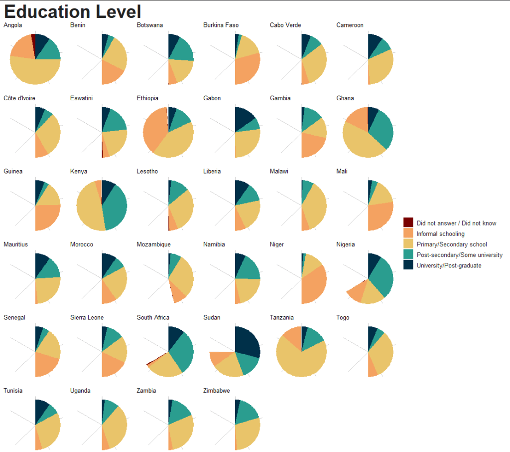
is_demo = Q36) -> ab_miniWe can visualise the educational status of the respondents across the countries in the survey.
In the codebook, the responses are coded as:
Question Number: Q97
Question: What is your highest level of education?
Variable Label: Q97. Education of respondent
Values: 0-9, 98, 99, -1
Value Labels: 0=No formal schooling, 1=Informal schooling only (including Koranic schooling), 2=Some primary schooling, 3=Primary school completed, 4=Intermediate school or some secondary school/high school, 5=Secondary school/high school completed, 6=Post-secondary qualifications, other than university, 7=Some university, 8=University completed, 9=Post-graduate, 98=Refused, 99=Don’t know, -1=Missing
Source: SAB
Before we graph the education levels, we can make sure they are in the order from the fewest to most years in education (rather than alphabetically).
edu_order <- c("Did not answer / Did not know",
               "Informal schooling",
               "Primary/Secondary school",
               "Post-secondary/Some university",
               "University/Post-graduate")
If we don’t add this following step, the pie charts end up incomplete this when we use facet_wrap()

So the next step is essential.
my_coord_polar <- coord_polar(theta = "y")
my_coord_polar$is_free <- function() TRUE
We can add some nice hex colors before we finish the graph.
traffic_light_palette <- c("#003049", "#2a9d8f", "#e9c46a", "#f4a261", "#780000")And create broader categories from the ten levels in the survey.
ab_mini %<>%
  filter(edu != -1) %>%
  mutate(edu_cat = case_when(
    edu %in% c(0, 1) ~ "Informal schooling",
    edu %in% c(2, 3, 4) ~ "Primary/Secondary school",
    edu %in% c(5, 6) ~ "Post-secondary/Some university",
    edu %in% c(7, 8, 9) ~ "University/Post-graduate",
    edu %in% c(98, 99) ~ "Did not answer / Did not know",
    TRUE ~ "Other")) %>%
  mutate(edu_cat = factor(edu_cat, levels = edu_order))
And finally, we can graph.
ab_mini %<>%
  mutate(edu_cat = factor(edu_cat, levels = edu_order)) %>%
  group_by(edu_cat, country_name) %>%
  count() %>%
  arrange(desc(n)) %>%
  ggplot(aes(x = "", y = n,
             fill = edu_cat), alpha = 0.75, color = "white",
         size = 1) +
  geom_bar(stat = "identity", width = 1) +
  my_coord_polar +
  theme_void() +
  facet_wrap(~country_name, scales = "free") +
  theme(aspect.ratio = 1) +
  labs(title = "Education Level")  +
  scale_fill_manual(values = rev(traffic_light_palette)) +
  my_theme() +
  theme(
    legend.text = element_text(size = 10),
    legend.position = "right",
    axis.text = element_blank(),
    axis.text.y = element_blank(),
    axis.text.x = element_blank(),
    axis.title = element_blank(),
    axis.ticks = element_blank(),
    strip.background = element_blank(),
strip.text = element_text(size = 10)) 
We can reorganise the order of the pie charts according to a specific value. In this case, we will organise from highest percentage of respondents with university-level education to lowest.
uni_order <- c("Sudan", "Gabon", "South Africa", "Mauritius", "Liberia", "Angola", "Tunisia", "Morocco", "Cameroon", "Kenya", "Nigeria", "Botswana", "Ghana", "Namibia", "Côte d'Ivoire", "Cabo Verde", "Togo", "Guinea", "Eswatini", "Ethiopia", "Senegal", "Benin","Tanzania", "Sierra Leone", "Zimbabwe", "Zambia", "Mali", "Burkina Faso", "Gambia", "Uganda", "Lesotho", "Mozambique", "Niger", "Malawi") And when we add the mutate(uni_country = factor(country_name, levels = uni_order)) line and replace all instances of country_name with uni_country, we can change the order of pie charts.
ab_mini %>%
  mutate(uni_country = factor(country_name, levels = uni_order)) %>%
  group_by(edu_cat, uni_country) %>%
  count() %>%
  arrange(desc(n)) %>%
  ggplot(aes(x = "", y = n,
             fill = edu_cat), alpha = 0.75, color = "white",
         size = 1) +
  geom_bar(stat = "identity", width = 1) +
  my_coord_polar +
  theme_void() +
  facet_wrap(~uni_country, scales = "free") +
  theme(aspect.ratio = 1) +
  labs(title = "Education Level")  +
  scale_fill_manual(values = rev(traffic_light_palette)) +
  my_theme() +
  theme(
    legend.text = element_text(size = 10),
    legend.position = "right",
    axis.text = element_blank(),
    axis.text.y = element_blank(),
    axis.text.x = element_blank(),
    axis.title = element_blank(),
    axis.ticks = element_blank(),
    strip.background = element_blank(),
strip.text = element_text(size = 10)) 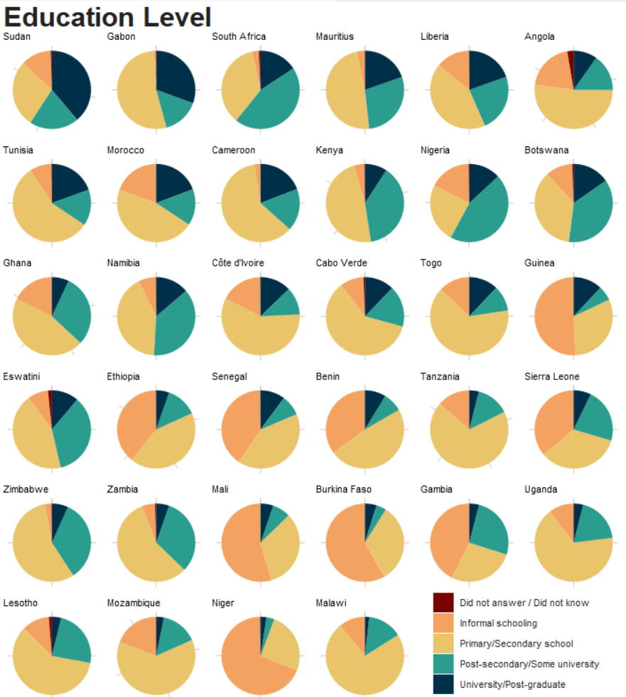
If we look at Sudan, we see that a large percentage of the respondents have a university degree. This is very different from the actual population.
https://idea.usaid.gov/cd/sudan/education
In a later blog, we will look at the survey weights that we can use in R. There are two weights supplied by the Afrobarometer dataset.
Hopefully, this accounts for the education level oversampling.
Next, we can create bard charts to compare countries and a lollipop plot to compare the responses of men and women to the question:
“How often, if ever, are people like you treated unfairly by the government based on your economic status, that is, how rich or poor you are?”
The respondents are as followed:
Value Labels: 0=Never, 1=Sometimes, 2=Often, 3=Always, 8=Refused, 9=Don’t know, -1=Missing
All the labels to the Likert questions are the following four categories. So we can feed this function in to our graphs to label the bar charts.
map_to_labels <- function(numeric_value) {
  case_when(
    numeric_value == 0 ~ "Never",
    numeric_value == 1 ~ "Sometimes",
    numeric_value == 2 ~ "Often",
    numeric_value == 3 ~ "Always",
    TRUE ~ as.character(numeric_value))
}
First, a simple histogram.
ab_mini %>%
  filter(govt_fair < 8) %>%
  ggplot(aes(x = govt_fair)) +
  geom_histogram(aes(fill = as.factor(govt_fair)), binwidth = 1, color = "black",
                 size = 2,
                 alpha = 0.5) +
  labs(title = "Average belief government treats respondents unfairly",
       x = " ",
       y = "Frequency") +
  scale_x_continuous(breaks = 0:3,
                     labels = map_to_labels(0:3)) +
  scale_fill_manual(values = traffic_light_palette) +
  my_theme() +
  theme(legend.position = "none")
We can use facet_wrap() again to compare countries:
ab_mini %>%
  filter(govt_fair < 8) %>%
  ggplot(aes(x = govt_fair)) +
  geom_histogram(aes(fill = as.factor(govt_fair)),
                 binwidth = 1, color = "black",
                 size = 1,
                 alpha = 0.5) +
  labs(title = "Average belief government treats respondents unfairly",
       x = " ", y = "Frequency") +
  scale_fill_manual(values = traffic_light_palette) +
  scale_x_continuous(breaks = 0:3, labels = map_to_labels(0:3)) +
  my_theme() +
  theme(legend.position = "none",
        axis.text.y = element_text(size = 10),
        axis.text.x = element_text(size = 10),
        axis.title.y =element_text(size = 15),
        strip.text = element_text(size = 10)) +
  facet_wrap(~country_name, scales = "free_y",
             ncol = 5)
And finally we can look at geom_segment to compare men and women across countries.
We have one extra step before we plot the geom_segments so that they are in order of highest level to lowest
ab_mini %>%
  group_by(country_name, gender) %>%
  summarise(mean_govt_fair = mean(govt_fair, na.rm = TRUE)) %>%
  ungroup() %>%
  pivot_wider(names_from = gender,
              values_from = mean_govt_fair) %>%
  select(country_name, male = `1`, female = `2`) %>%
  rowwise() %>%
  mutate(mymean = mean(c(male, female) )) %>%
  arrange(mymean) %>%
  mutate(country_name = as.factor(country_name)) -> ab_lollipop
After we arrange according to the highest to lowest mean levels per country, we can graph:
ab_lollipop %>%
  ggplot() +
  geom_segment( aes(x = country_name, xend = country_name,
                    y = female, yend = male), color = "#000814", alpha = 0.5, size = 2) +
  geom_point( aes(x = country_name, y = female), color = "#780000", alpha = 0.75, size = 5) +
  geom_point( aes(x = country_name, y = male), color = "#003049", alpha = 0.75, size = 5) +
  coord_flip() +
  labs(title = "Average belief government treats respondents unfairly",
       x = " ",
       y = "I am treated unfairly by government based on economic status") +
  my_theme() +
  theme(axis.text.y = element_text(size = 10),
axis.title.x =element_text(size = 20)) 
Finally we will graph out the variables on a map of Africa.
We can download the map coordinates with the rnaturalearth package.
Click here to read more about this package.
We can use the ne_countries() function to download the map and just just the continent of Africa.
ne_countries(scale = "medium", returnclass = "sf") %>%
  filter(region_un == "Africa") %>%
  select(geometry, name_long) -> map
We can look at the average age of the survey respondents in the countries.
Before we map out the average age per country, we calculate the overall age in the full survey. This is so we can use it as the midpoint for the color gradients for our map!
ab_mid <- ab %>%
  summarise(mid = mean(age, na.rm = TRUE))
37.3 years
We calculate the age for each country and graph out the map
ab_mini %>%
  filter(age < 100) %>%
  group_by(iso) %>%
  summarise(mean_age = mean(age, na.rm = TRUE)) %>%
  ungroup() %>%
  right_join(map, by = "iso") %>%
  ggplot() +
  geom_sf(aes(geometry = geometry, fill = mean_age),
          position = "identity", color = "#333333", linewidth = 0.75) +
  scale_fill_gradient2(midpoint = ab_mid$mid, low = "#457b9d", mid = "white",
                       high = "#780000", space = "Lab") + my_map_theme() +
  labs(title = "Average age of survey respondents"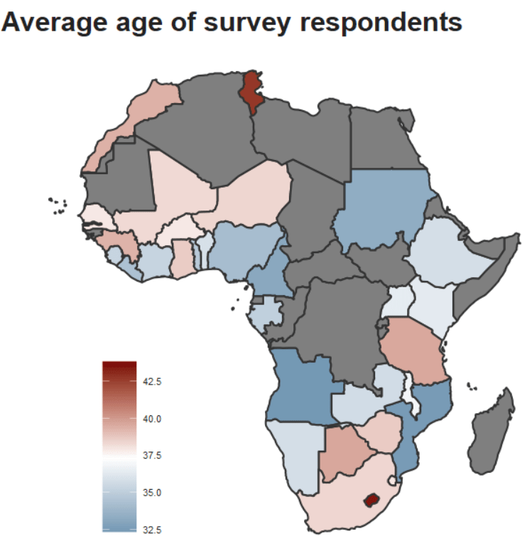

We can compare country means to the overall survey means on the question about how the respondents see the economy in the future.
Question Number: Q6B
Question: Looking ahead, do you expect economic conditions in this country to be better or worse in twelve months’ time?
Value Labels:
1=Much worse,
2=Worse,
3=Same,
4=Better,
5=Much better,
8=Refused,
9=Don’t know,
-1=Missing
We take the above question and filter out 8 and 9:
ab_mini %>%
  group_by(state_econ_future) %>%
  count()
# A tibble: 5 × 2
# Groups:   state_econ_future [5]
  state_econ_future     n
              <dbl> <int>
1                 1  6396
2                 2  7275
3                 3  6640
4                 4 16454
5                 5  5595
We can add the labels as a new string variable in factor form.
value_labels <- c("1" = "Much worse", "2" = "Worse", "3" = "Same", "4" = "Better", "5" = "Much better")

ab_mini %<>%
  filter(state_econ_future < 8) %>%
  mutate(state_econ_future_factor = factor(state_econ_future, levels = as.character(1:5), labels = value_labels))
Next we calculate the mean for each country – state_econ_future_mean – and then a grand mean for all respondents in the survey regardless of their country – grand_state_econ_mean.
ab_demo_gdp %>%
  group_by(country_name) %>%
  mutate(state_econ_future_mean = mean(state_econ_future)) %>%
  ungroup() %>%
  mutate(grand_state_econ_mean = mean(state_econ_future)) %>%
  distinct(country_name, state_econ_future_mean, grand_state_econ_mean) %>%
  mutate(diff_grand_country_mean =  state_econ_future_mean - grand_state_econ_mean) %>%
  arrange(desc(diff_grand_country_mean)) -> econ_means
If we want to add flags, we add ISO 2 character codes (in lower text, not in capital letters).
Click here to read more about the ggflags package!
econ_means %<>%
  mutate(iso2 = tolower(countrycode(country_name, "country.name", "iso2c")))
And we use the geom_hline() to add a vertical line for the overall grand survey mean.
The geom_segment() allows us to draw the horizontal line from the mean of the country to the overall grand mean.
Click here to read more about using the geom_segment() layer in ggplot
econ_means %>%
  ggplot(aes(x = reorder(country_name, state_econ_future_mean),
             y = state_econ_future_mean)) +
  geom_point(alpha = 0.7, width = 0.15, size = 5) +
  geom_hline(aes(yintercept = grand_state_econ_mean), color = "black", size = 2) +
  geom_segment(aes(x = country_name,
                   xend = country_name,
                   yend = grand_state_econ_mean,
                   color = ifelse(state_econ_future_mean > grand_state_econ_mean,
                                  "#008000" , "#E4002B"), alpha = 0.5), size = 4) +
  ggflags::geom_flag(aes(x = country_name, y = 1.75, country = iso2), size = 6) +
  coord_flip() +
  scale_color_manual(values = c("#008000", "#E4002B")) +
  my_theme() +
  theme(legend.position = "none") +
  labs(title = "Economy will be better in 12 months",
       subtitle = "Afrobarometer, 2022",
       x = " ",
       y = " ")


