How to graph model variables with the tidy package in R

Packages we will need:

library(tidyverse)
library(broom)
library(stargazer)
library(janitor)
library(democracyData)
library(WDI)

We will make a linear regression model and graph the coefficients to show which variables are statistically significant in the regression with ggplot.

First we will download some variables from the World Bank Indicators package.

Click here to read more about the WDI package.

Download WorldBank data with WDI package in R

We will use Women Business and the Law Index Score as our dependent variable.

The index measures how laws and regulations affect women’s economic opportunity. Overall scores are calculated by taking the average score of each index (Mobility, Workplace, Pay, Marriage, Parenthood, Entrepreneurship, Assets and Pension), with 100 representing the highest possible score.

And then a few independent variables for the model

women_business = WDI(indicator = "SG.LAW.INDX")

gdp_percap = WDI(indicator = "NY.GDP.PCAP.KD")
pop <- WDI(indicator = "SP.POP.TOTL") 
mil_spend_gdp = WDI(indicator = "MS.MIL.XPND.ZS")
mortality = WDI(indicator = "SP.DYN.IMRT.IN")

We will merge them all together and rename the columns with inner_join()

women_business %>%
  filter(year > 1999) %>% 
  inner_join(mortality) %>% 
  inner_join(mil_spend_gdp) %>% 
  inner_join(gdp_percap) %>% 
  inner_join(pop) %>% 
  inner_join(mortality) %>% 
  select(country, year, iso2c,
         pop = SP.POP.TOTL,
         fem_bus = SG.LAW.INDX, 
         mortality = SP.DYN.IMRT.IN,
         gdp_percap = NY.GDP.PCAP.KD,
         mil_gdp = MS.MIL.XPND.ZS) -> wdi

We will remove all NA values and take a summary of all the variables.

Finally, we will filter out al the variables that are not countries according to the Correlates of War project.

  wdi %>%  mutate_all(~ifelse(is.nan(.), NA, .)) %>% 
  select(-year) %>% 
  group_by(country, iso2c) %>% 
  summarize(across(where(is.numeric), mean,  
                   na.rm = TRUE, .names = "mean_{col}")) %>% 
  ungroup() %>% 
  mutate(cown = countrycode::countrycode(iso2c, "iso2c", "cown")) %>% 
  filter(!is.na(cown)) -> wdi_summary

Next we will also download Freedom House values from the democracyData package.

Visualise DemocracyData with graphs and maps

fh <- download_fh()

fh %>% 
  group_by(fh_country) %>% 
  filter(year > 1999) %>% 
  summarise(mean_fh = mean(fh_total, na.rm = TRUE)) %>% 
  mutate(cown = countrycode::countrycode(fh_country, "country.name", "cown")) %>% 
  mutate_all(~ifelse(is.nan(.), NA, .)) %>% 
  filter(!is.na(cown))  -> fh_summary

If you want to find resources for more data packages, click here.

Top R packages for downloading political science and economics datasets

We merge the Freedom House and World Bank data

fh_summary %>%
  inner_join(wdi_summary, by = "cown") %>% 
  select (-c(cown, iso2c, fh_country)) -> wdi_fh

We can look at the summarise of all the variables with the skimr package.

Summarise data with skimr package in R

wdi_fh %>% 
  skim()

And we will take the log of some of the following variables:

wdi_fh %<>% 
  mutate(log_mean_pop = log10(mean_pop),
         log_mean_gdp_percap = log10(mean_gdp_percap),
         log_mean_mil_gdp = log10(mean_mil_gdp)) %>% 
  select(!c(country, mean_pop, mean_gdp_percap, mean_mil_gdp))

Next, we run a quick linear regression model

wdi_fh %>% 
  lm(mean_fem_bus ~ ., data = .) -> my_model

We can print the model output with the stargazer package

my_model %>%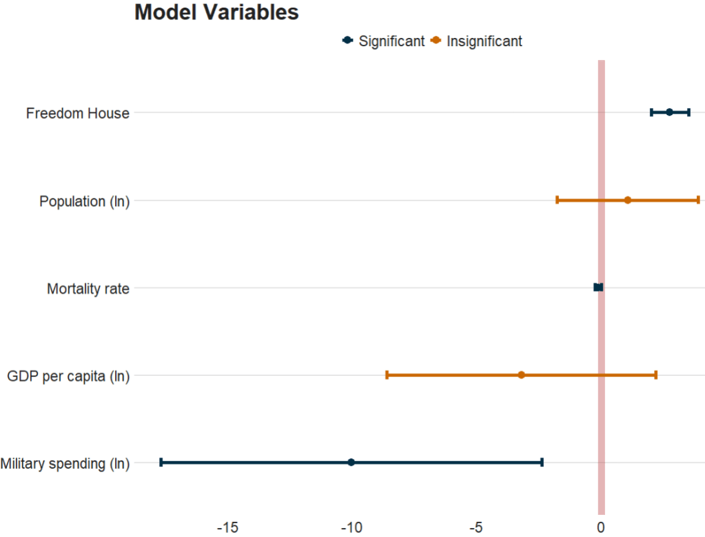 
  stargazer(type = "html")


	Dependent variable:

	mean_fem_bus

mean_fh	2.762^***
	(0.381)

mean_mortality	-0.131^**
	(0.065)

log_mean_pop	1.065
	(1.434)

log_mean_gdp_percap	-3.201
	(2.735)

log_mean_mil_gdp	-10.038^**
	(3.870)

Constant	61.030^***
	(16.263)


Observations	154
R²	0.566
Adjusted R²	0.551
Residual Std. Error	11.912 (df = 148)
F Statistic	38.544^*** (df = 5; 148)

Note:	^p<0.1; ^p<0.05; ^**p<0.01

And we will use the tidy() function from the broom package to extract the estimates and confidence intervals from the model

my_model %>%
  tidy(., conf.int = TRUE) %>% 
  filter(term != "(Intercept)") %>% 
  janitor::clean_names() %>% 
  mutate(term = ifelse(term == "log_mean_mil_gdp", "Military spending (ln)",
    ifelse(term == "log_mean_gdp_percap", "GDP per capita (ln)",
    ifelse(term == "log_mean_pop", "Population (ln)",
    ifelse(term == "mean_mortality", "Mortality rate",
    ifelse(term == "mean_fh", "Freedom House", "Other")))))) -> tidy_model

And we can plot the tidy values

tidy_model %>% 
  ggplot(aes(x = reorder(term, estimate), y = estimate)) +
  geom_hline(yintercept = 0, color = "#bc4749", size = 4, alpha = 0.4) +
  geom_errorbar(aes(ymin = conf_low, ymax = conf_high,
  color = ifelse(conf_low * conf_high > 0, "#023047", 
  ifelse(term == "Mortality rate", "#ca6702", "#ca6702"))), width = 0.1, size = 2) +
  geom_point(aes(color = ifelse(conf_low * conf_high > 0, "#023047", 
  ifelse(term == "Mortality rate", "#ca6702", "#ca6702"))), size = 4) + 
coord_flip() +
  scale_color_manual(labels = c("Significant", "Insignificant"), values = c("#023047", "#ca6702")) +
labs(title = "Model Variables", x = "", y = "", caption = "Source: Your Data Source") + bbplot::bbc_style()