Check linear regression assumptions with gvlma package in R

Packages we will need:

library(gvlma)

gvlma stands for Global Validation of Linear Models Assumptions. See Peña and Slate’s (2006) paper on the package if you want to check out the math!

Linear regression analysis rests on many MANY assumptions. If we ignore them, and these assumptions are not met, we will not be able to trust that the regression results are true.

Luckily, R has many packages that can do a lot of the heavy lifting for us. We can check assumptions of our linear regression with a simple function.

So first, fit a simple regression model:

 data(mtcars)
 summary(car_model <- lm(mpg ~ wt, data = mtcars)) 

We then feed our car_model into the gvlma() function:

gvlma_object <- gvlma(car_model)

• Global Stat checks whether the relationship between the dependent and independent relationship roughly linear. We can see that the assumption is met.

• Skewness and kurtosis assumptions show that the distribution of the residuals are normal.

• Link function checks to see if the dependent variable is continuous or categorical. Our variable is continuous.

• Heteroskedasticity assumption means the error variance is equally random and we have homoskedasticity!

Often the best way to check these assumptions is to plot them out and look at them in graph form.

Next we can plot out the model assumptions:

plot.gvlma(glvma_object)

The relationship is a negative linear relationship between the two variables.

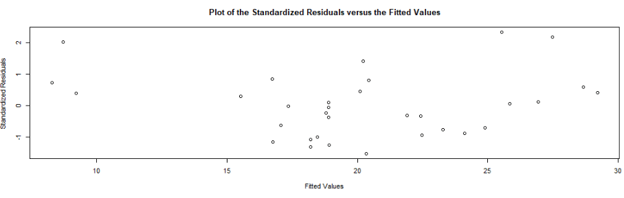
This scatterplot of residuals on the y axis and fitted values (estimated responses) on the x axis. The plot is used to detect non-linearity, unequal error variances, and outliers.

As explained in this Penn State webpage on interpreting residuals versus fitted plots:

• The residuals “bounce randomly” around the 0 line. This suggests that the assumption that the relationship is linear is reasonable.
• The residuals roughly form a “horizontal band” around the 0 line. This suggests that the variances of the error terms are equal.
• No one residual “stands out” from the basic random pattern of residuals. This suggests that there are no outliers.

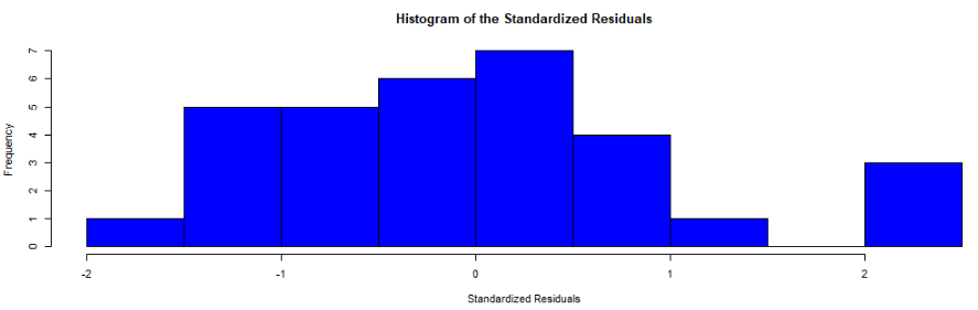
In this histograpm of standardised residuals, we see they are relatively normal-ish (not too skewed, and there is a single peak).

Next, the normal probability standardized residuals plot, Q-Q plot of sample (y axis) versus theoretical quantiles (x axis). The points do not deviate too far from the line, and so we can visually see how the residuals are normally distributed.

Click here to check out the CRAN pdf for the gvlma package.

References

Peña, E. A., & Slate, E. H. (2006). Global validation of linear model assumptions. Journal of the American Statistical Association, 101(473), 341-354.