We use the grid_latin_hypercube() function from the dials package in R is used to generate a sampling grid for tuning hyperparameters using a Latin hypercube sampling method.
Latin hypercube sampling (LHS) is a way to generate a sample of plausible, semi-random collections of parameter values from a distribution.
This method is used to ensure that each parameter is uniformly sampled across its range of values. LHS is systematic and stratified, but within each stratum, it employs randomness.
Inside the grid_latin_hypercube() function,we can set the ranges for the model parameters,
trees(range = c(500, 1500))
This parameter specifies the number of trees in the model
We can set a sampling range from 500 to 1500 trees.
tree_depth(range = c(3, 10))
This defines the maximum depth of each tree
We set values ranging from 3 to 10.
learn_rate(range = c(0.01, 0.1))
This parameter controls the learning rate, or the step size at each iteration while moving toward a minimum of a loss function.
It’s specified to vary between 0.01 and 0.1.
size = 20
We want the Latin Hypercube Sampling to generate 20 unique combinations of the specified parameters. Each of these combinations will be used to train a model, allowing for a systematic exploration of how different parameter settings impact model performance.
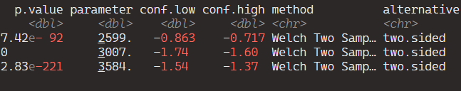
So next, we will combine our recipe, model specification, and resampling method in a workflow, and use tune_grid() to find the best hyperparameters based on RMSE.
The tune_grid() function does the hyperparameter tuning. We will make different combinations of hyperparameters specified in grid using cross-validation.
After tuning, we can extract and examine the best models.
show_best(tuning_results, metric = "rmse")
  trees tree_depth learn_rate .metric .estimator  mean     n std_err .config
  <int>      <int>      <dbl> <chr>   <chr>      <dbl> <int>   <dbl> <chr>
1   593          4       1.11 rmse    standard   0.496    10  0.0189 Preprocessor1_Model03
2   677          3       1.25 rmse    standard   0.500    10  0.0216 Preprocessor1_Model02
3  1296          6       1.04 rmse    standard   0.501    10  0.0238 Preprocessor1_Model09
4  1010          5       1.15 rmse    standard   0.501    10  0.0282 Preprocessor1_Model08
5  1482          5       1.05 rmse    standard   0.502    10  0.0210 Preprocessor1_Model05
The best model is model number 3!
Finally, we can plot it out.
We use collect_metrics() to pull out the RMSE and other metrics from our samples.
It automatically aggregates the results across all resampling iterations for each unique combination of model hyperparameters, providing mean performance metrics (e.g., mean accuracy, mean RMSE) and their standard errors.
In this blog post, we are going to run boosted decision trees with xgboost in tidymodels.
Boosted decision trees are a type of ensemble learning technique.
Ensemble learning methods combine the predictions from multiple models to create a final prediction that is often more accurate than any single model’s prediction.
The ensemble consists of a series of decision trees added sequentially, where each tree attempts to correct the errors of the preceding ones.
Similar to the previous blog, we will use Varieties of Democracy data and we will examine the relationship between judicial corruption and public sector theft.
mode specifies the type of predictive modeling that we are running.
Common modes are:
"regression" for predicting numeric outcomes,
"classification" for predicting categorical outcomes,
"censored" for time-to-event (survival) models.
The mode we choose is regression.
Next we add the number of trees to include in the ensemble.
More trees can improve model accuracy but also increase computational cost and risk of overfitting. The choice of how many trees to use depends on the complexity of the dataset and the diminishing returns of adding more trees.
We will choose 1000 trees.
tree_depth indicates the maximum depth of each tree. The depth of a tree is the length of the longest path from a root to a leaf, and it controls the complexity of the model.
Deeper trees can model more complex relationships but also increase the risk of overfitting. A smaller tree depth helps keep the model simpler and more generalizable.
Our model is quite simple, so we can choose 3.
When your model is very simple, for instance, having only one independent variable, the need for deep trees diminishes. This is because there are fewer interactions between variables to consider (in fact, no interactions in the case of a single variable), and the complexity that a model can or should capture is naturally limited.
For a model with a single predictor, starting with a lower max_depth value (e.g., 3 to 5) is sensible. This setting can provide a balance between model simplicity and the ability to capture non-linear relationships in the data.
The best way to determine the optimal max_depth is with cross-validation. This involves training models with different values of max_depth and evaluating their performance on a validation set. The value that results in the best cross-validated metric (e.g., RMSE for regression, accuracy for classification) is the best choice.
We will look at RMSE at the end of the blog.
Next we look at the min_n, which is the minimum number of data points allowed in a node to attempt a new split. This parameter controls overfitting by preventing the model from learning too much from the noise in the training data. Higher values result in simpler models.
We choose min_n of 10.
loss_reduction is the minimum loss reduction required to make a further partition on a leaf node of the tree. It’s a way to control the complexity of the model; larger values result in simpler models by making the algorithm more conservative about making additional splits.
We input a loss_reduction of 0.01.
A low value (like 0.01) means that the model will be more inclined to make splits as long as they provide even a slight improvement in loss reduction.
This can be advantageous in capturing subtle nuances in the data but might not be as critical in a simple model where the potential for overfitting is already lower due to the limited number of predictors.
sample_size determines the fraction of data to sample for each tree. This parameter is used for stochastic boosting, where each tree is trained on a random subset of the full dataset. It introduces more variation among the trees, can reduce overfitting, and can improve model robustness.
Our sample_size is 0.5.
While setting sample_size to 0.5 is a common practice in boosting to help with overfitting and improve model generalization, its optimality for a model with a single independent variable may not be suitable.
We can test different values through cross-validation and monitoring the impact on both training and validation metrics
mtry indicates the number of variables randomly sampled as candidates at each split. For regression problems, the default is to use all variables, while for classification, a commonly used default is the square root of the number of variables. Adjusting this parameter can help in controlling model complexity and overfitting.
For this regression, our mtry will equal 2 variables at each split
learn_rate is also known as the learning rate or shrinkage. This parameter scales the contribution of each tree.
We will use a learn_rate = 0.01.
A smaller learning rate requires more trees to model all the relationships but can lead to a more robust model by reducing overfitting.
Finally, engine specifies the computational engine to use for training the model. In this case, "xgboost" package is used, which stands for eXtreme Gradient Boosting.
When to use each argument:
Mode: Always specify this based on the type of prediction task at hand (e.g., regression, classification).
Trees, tree_depth, min_n, and loss_reduction: Adjust these to manage model complexity and prevent overfitting. Start with default or moderate values and use cross-validation to find the best settings.
Sample_size and mtry: Use these to introduce randomness into the model training process, which can help improve model robustness and prevent overfitting. They are especially useful in datasets with a large number of observations or features.
Learn_rate: Start with a low to moderate value (e.g., 0.01 to 0.1) and adjust based on model performance. Smaller values generally require more trees but can lead to more accurate models if tuned properly.
Engine: Choose based on the specific requirements of the dataset, computational efficiency, and available features of the engine.
The tidymodels framework in R is a collection of packages for modeling.
Within tidymodels, the parsnip package is primarily responsible for specifying models in a way that is independent of the underlying modeling engines. The set_engine() function in parsnip allows users to specify which computational engine to use for modeling, enabling the same model specification to be used across different packages and implementations.
In this blog series, we will look at some commonly used models and engines within the tidymodels package
Linear Regression (lm): The classic linear regression model, with the default engine being stats, referring to the base R stats package.
Logistic Regression (logistic_reg): Used for binary classification problems, with engines like stats for the base R implementation and glmnet for regularized regression.
Random Forest (rand_forest): A popular ensemble method for classification and regression tasks, with engines like ranger and randomForest.
Boosted Trees (boost_tree): Used for boosting tasks, with engines such as xgboost, lightgbm, and catboost.
Decision Trees (decision_tree): A base model for classification and regression, with engines like rpart and C5.0.
K-Nearest Neighbors (nearest_neighbor): A simple yet effective non-parametric method, with engines like kknn and caret.
Principal Component Analysis (pca): For dimensionality reduction, with the stats engine.
Lasso and Ridge Regression (linear_reg): For regression with regularization, specifying the penalty parameter and using engines like glmnet.