
Packages we will use:
library(tidyverse)
library(rvest)
library(janitor)
library(magrittr)
library(ggparliament)
library(ggbump)
library(bbplot)
I am an Irish person living abroad. I did NOT follow the elections last year. So, as penance (as I just mentioned, I am Irish and therefore full of phantom Catholic guilt for neglecting political news back home), we will be graphing some of the election data and familiarise ourselves with the new contours of Irish politics in this blog.
Click here to visit the wikipedia page we will be scraping with the rvest package.
Click here to read more about the rvest package for webscraping.
The data we want is in the 11th table on the page:

The columns that we will want are the Party and the Elected 2024 columns.
So using the read_html() function, we can feed in the URL, save all the tables with html_table() and then only keep the eleventh table with `[[`(11)
read_html("https://en.wikipedia.org/wiki/2024_Irish_general_election") %>%
  html_table(header = TRUE, fill = TRUE) %>%
  `[[`(11) -> dail_2024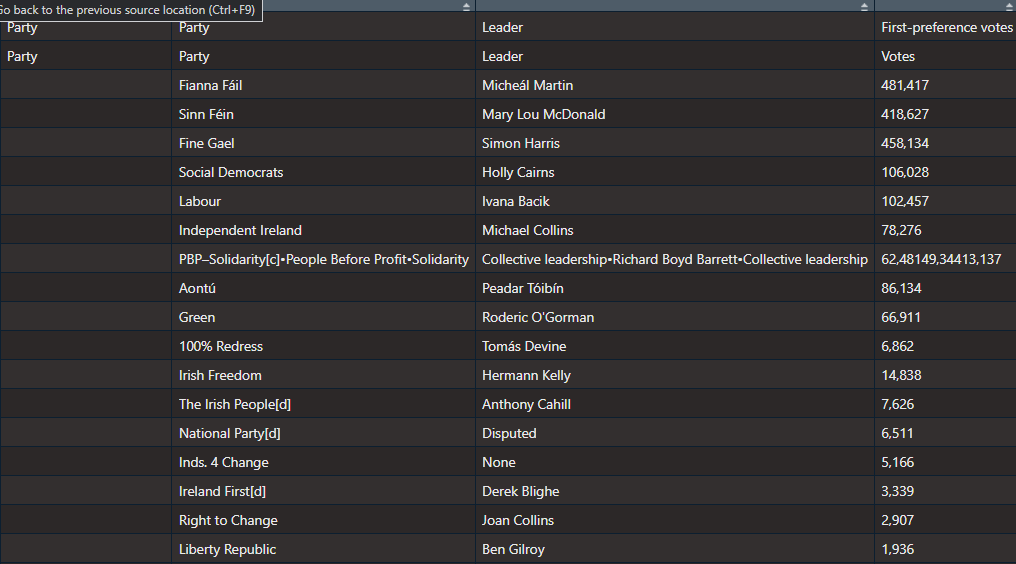
It’s a bit of a hot mess at this stage.
Right now, all the variable names are empty.
We can use the row_to_names() function from the janitor package. This moves a row up to became the variable names. Also we can use clean_names() (also a janitor package staple) to make every variable lowercase snake_case with underscores.
dail_2024 %<>%
  row_to_names(row_number = 2) %>%
  clean_names() %>%
As you can see in the table above, the PBP cell is very crowded. This is due to the fact that many similar left-wing parties formed a loose coaltion when campaigning.
Because they are all in one cell, every number was shoved together without spaces. So instead of each party in the loose grouping, it was all added together. It makes the table wholly incorrect; the PBP coalition did not win trillions of votes.
Things like this highlights the importance of always checking the raw data after web scraping.
So I just brute recode the value according to what is actually on the Wiki page.
dail_2024 %<>%
  mutate(elected2024 = if_else(party_2 == "PBP–Solidarity[c]•People Before Profit•Solidarity", "3", elected2024))
Next we need to remove the annoying [footnotes in square brackets] on the page with some regex nonsense.
dail_2024 %<>%
  mutate(across(everything(), ~ str_replace(., "\\[.*$", "")))
And finally, we just need to select, rename and change the seat numbers from character to numeric
dail_2024 %<>%
  select(party = party_2, seats = elected2024)  %>%
  mutate(seats= parse_number(seats))
Next, we just need to graph it out with the geom_parliament_seats() layer of the ggplot graph with ggparliament package.
Click here to read more about the ggparliament package:
First, we generate the circle coordinates
dail_2024_coord <- parliament_data(election_data = dail_2024,
                   type = "semicircle",
                   parl_rows = 6,
                   party_seats = dail_2024$seats_2024)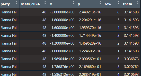
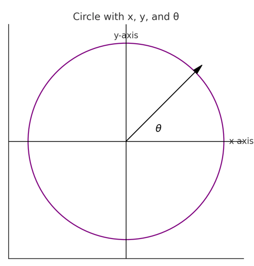
x: the horizontal position of a point in the semi-circle graph.
y: the vertical position of a point in the semi-circle graph.
row: The row or layer of the semi-circle in which the point (seat) is positioned. Rows are arranged from the base (row 1) to the top of the semi-circle.
theta: The angle (in radians) used to calculate the position of each seat in the semi-circle. It determines the angular placement of each point, starting at 0 radians (rightmost point of the semi-circle) and increasing counterclockwise to π\piπ radians (leftmost point of the semi-circle).
We want to have the biggest parties first and the smallest parties at the right of the graph
dail_elected %<>%
  mutate(party = fct_reorder(party, table(party)[party], .desc = TRUE))
and we can add some hex colors that represent the parties’ representative colours.
dail_elected_coord %<>%
  mutate(party_colour = case_when(party == "Fianna Fáil" ~ "#66bb66",
                       party == "Fine Gael" ~ "#6699ff",
                       party == "Green" ~ "#2fb66a",
                       party == "Labour" ~ "#e71c38",
                       party == "Sinn Féin" ~ "#326760",
                       party == "PBP–Solidarity" ~ "#e91d50",
                       party ==  "Social Democrats" ~ "#742a8b",
                       party == "Independent Ireland" ~ "#ee9f27",
                       party == "Aontú" ~ "#4f4e31",
                       party == "100% Redress" ~ "#8e2420"))
And we graph out the ggplot with the simple bbc_style() from the bbplot package
dail_elected_coord %>%
  ggplot(aes(x = x, y = y,
             colour = party)) +
  geom_parliament_seats(size = 13) +
  bbplot::bbc_style()  +
  ggtitle("34th Irish Parliament") +
  theme(text = element_text(size = 50),
        legend.title = element_blank(),
        axis.text.x = element_blank(),
        axis.text.y = element_blank())  +
  scale_colour_manual(values = dail_elected_coord$party_colour,
                      limits = dail_elected_coord$party)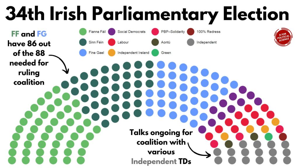
HONESTY TIME… I will admit, I replaced the title as well as the annotated text and arrows with Canva dot comm
Hell is … trying to incrementally make annotations to go to place we want via code. Why would I torment myself when drag-and-drop options are available for free.
Next, let’s compare this year with previous years
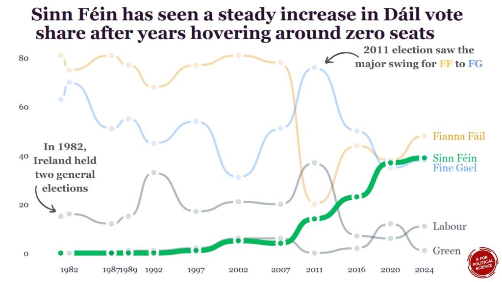
I was also hoping to try replicate this blog post about bump plots with highlighted labels from the r-graph-gallery website.
We can use this kind of graph to highlight a particular trend.
For example, the rise of Sinn Fein as a heavy-hitter in Irish politics.
We will need to go to many of the Wikipedia pages on the elections and scrape seat data for the top parties for each year.
Annoyingly, across the different election pages, the format is different so we have to just go by trial-and-error to find the right table for each election year and to find out what the table labels are for each given year.
Since going to many different pages ends up with repeating lots of code snippets, we can write a process_election_data() function to try cut down on replication.
process_election_data <- function(url, table_index, header_row, party_col, seats_col, top_parties, extra_mutate = NULL) {
  read_html(url) %>%
    html_table(header = TRUE, fill = TRUE) %>%
    `[[`(table_index) %>%
    row_to_names(row_number = header_row) %>%
    clean_names() %>%
    mutate(across(everything(), ~ str_replace(., "\\[.*$", ""))) %>%
    select(party = !!sym(party_col), seats = !!sym(seats_col)) %>%
    mutate(seats = parse_number(seats)) %>%
    filter(party %in% top_parties)
}
In this function, mutate(across(everything(), ~ str_replace(., "\\[.*$", ""))) removes all those annoying footnotes in square brackets from the Wiki table with regex code.
Annoyingly, the table for the 2024 election is labelled differently to the table with the 2016 results on le Wikipedia. So when we are scraping from each webpage, we will need to pop in a sliiiightly different string.
We can use the sym() and the !! to accomodate that.
When we type on !! (which the coder folks call bang-bang), this unquotes the string we feed in. We don’t want the function to treat our string as a string.
After this !! step, we can now add them as variables within the select() function.
We will only look at the biggest parties that have been on the scene since 1980s
top_parties <- c("Fianna Fáil", "Fine Gael", "Sinn Féin", "Labour Party", "Green Party")Now, we feed in the unique features that are unique for scraping each web page:
dail_2024 <- process_election_data(
  url = "https://en.wikipedia.org/wiki/2024_Irish_general_election
  table_index = 11,
  header_row = 2,
  party_col = "party_2",
  seats_col = "elected2024",
  top_parties = top_parties)

dail_2020 <- process_election_data(
  url = "https://en.wikipedia.org/wiki/2020_Irish_general_election",
  table_index = 10,
  header_row = 2,
  party_col = "party_2",
  seats_col = "elected2020",
  top_parties = top_parties)

dail_2016 <- process_election_data(
  url = "https://en.wikipedia.org/wiki/2016_Irish_general_election",
  table_index = 10,
  header_row = 3,
  party_col = "party_2",
  seats_col = "elected2016_90",
  top_parties = top_parties)

dail_2011 <- process_election_data(
  url = "https://en.wikipedia.org/wiki/2011_Irish_general_election",
  table_index = 14,
  header_row = 2,
  party_col = "party_2",
  seats_col = "t_ds",
  top_parties = top_parties)

dail_2007 <- process_election_data(
  url = "https://en.wikipedia.org/wiki/2007_Irish_general_election",
  table_index = 8,
  header_row = 2,
  party_col = "party_2",
  seats_col = "seats",
  top_parties = top_parties)

dail_2002 <- process_election_data(
  url = "https://en.wikipedia.org/wiki/2002_Irish_general_election",
  table_index = 8,
  header_row = 2,
  party_col = "party_2",
  seats_col = "seats",
  top_parties = top_parties)

dail_1997 <- process_election_data(
  url = "https://en.wikipedia.org/wiki/1997_Irish_general_election",
  table_index = 9,
  header_row = 2,
  party_col = "party_2",
  seats_col = "seats",
  top_parties = top_parties)

dail_1992 <- process_election_data(
  url = "https://en.wikipedia.org/wiki/1992_Irish_general_election",
  table_index = 6,
  header_row = 2,
  party_col = "party_2",
  seats_col = "seats",
  top_parties = top_parties)

dail_1989 <- process_election_data(
  url = "https://en.wikipedia.org/wiki/1989_Irish_general_election",
  table_index = 5,
  header_row = 2,
  party_col = "party_2",
  seats_col = "seats",
  top_parties = top_parties)

dail_1987 <- process_election_data(
  url = "https://en.wikipedia.org/wiki/1987_Irish_general_election",
  table_index = 5,
  header_row = 2,
  party_col = "party_2",
  seats_col = "seats",
  top_parties = top_parties)

dail_1982_11 <- process_election_data(
  url = "https://en.wikipedia.org/wiki/November_1982_Irish_general_election",
  table_index = 5,
  header_row = 2,
  party_col = "party_2",
  seats_col = "seats",
  top_parties = top_parties)

dail_1982_2 <- process_election_data(
  url = "https://en.wikipedia.org/wiki/February_1982_Irish_general_election",
  table_index = 5,
  header_row = 2,
  party_col = "party_2",
  seats_col = "seats",
  top_parties = top_parties)
After we scraped every election, we can join them together
dail_years <- dail_2024 %>%
  left_join(dail_2020, by = c("party")) %>%
  left_join(dail_2016, by = c("party")) %>%
  left_join(dail_2011, by = c("party")) %>%
  left_join(dail_2007, by = c("party")) %>%
  left_join(dail_2002, by = c("party")) %>%
  left_join(dail_1997, by = c("party")) %>%
  left_join(dail_1992, by = c("party")) %>%
  left_join(dail_1989, by = c("party")) %>%
  left_join(dail_1987, by = c("party")) %>%
  left_join(dail_1982_11, by = c("party")) %>%
  left_join(dail_1982_2, by = c("party"))
Or I can use a list and iterative left joins.
dail_list <- list(
  dail_2024,
  dail_2020,
  dail_2016,
  dail_2011,
  dail_2007,
  dail_2002,
  dail_1997,
  dail_1992,
  dail_1989,
  dail_1987,
  dail_1982_11,
  dail_1982_2)

dail_years <- reduce(dail_list, left_join, by = "party")
For the x axis ticks, we can quickly make a vector of all the election years we want to highlight on the graph.
election_years <- c(2024, 2020, 2016, 2011, 2007, 2002, 1997, 1992, 1989, 1987, 1982)Next we pivot the data to long format:
dail_years %>% pivot_longer(
  cols = starts_with("seats_"),
  names_to = "year",
  names_prefix = "seats_",
  values_to = "seats") -> dail_longer
Then we can add specific hex colours for the main parties.
dail_longer %<>%
  mutate(color = ifelse(party == "Sinn Féin", "#2fb66a",
         ifelse(party == "Fine Gael","#6699ff",
         ifelse(party == "Fianna Fáil","#ee9f27","#495051"))))
Next, we can create a final_positions data.frame so that can put the names of the political parties at the end of the trend line instead of having a legend floating at top of the graph.
final_positions <_ dail_longer %>%
  group_by(party) %>%
  filter(year == max(year))  %>%
  mutate(color = ifelse(party == "Sinn Féin", "#2fb66a",
         ifelse(party == "Fine Gael","#6699ff",
         ifelse(party == "Fianna Fáil","#ee9f27", "#495051")))
Click here to read more about the ggbump package
dail_longer %>%
  ggplot(aes(x = year, y = seats, group = party)) +

  geom_bump(aes(color = color,
           alpha = ifelse(party == "Sinn Féin", 0.5, 0.2),
           linewidth = ifelse(party == "Sinn Féin", 0.8, 0.7)),
            smooth = 5) +

  geom_text(data = final_positions,
            aes(color = color,
            y = ifelse(party == "Fine Gael", seats - 3, seats),
            label = party,
            family = "Georgia"),
            x = x_position + 1.5,
            hjust = 0,
            size = 10) +

  geom_point(color = "white",
             size = 6,
             stroke = 3) +

  geom_point(aes(color = color,
             alpha = ifelse(party == "Sinn Féin", 0.5, 0.1)),
             size = 4) +

  scale_linewidth_continuous(range = c(2, 5)) +

  scale_alpha_continuous(range = c(0.2, 1)) +

  bbplot::bbc_style()  +

  theme(legend.position = "none",
        plot.title = element_text(size = 48)) +

  scale_color_identity() +

  scale_x_continuous(limits = c(1980, 2030), breaks = election_years) +

  labs(title = "Sinn Féin has seen a steady increase in Dáil vote\n share after years hovering around zero seats")


