Analyse Pseudo-R2, VIF scores and robust standard errors for generalised linear models in R

This blog post will look at a simple function from the jtools package that can give us two different pseudo R2 scores, VIF score and robust standard errors for our GLM models in R

Packages we need:

library(jtools)
library(tidyverse)

From the Varieties of Democracy dataset, we can examine the v2regendtype variable, which codes how a country’s governing regime ends.

It turns out that 1994 was a very coup-prone year. Many regimes ended due to either military or non-military coups.

We can extract all the regimes that end due to a coup d’etat in 1994. Click here to read the VDEM codebook on this variable.

vdem_2 <- vdem %>% 
  dplyr::filter(vdem$year == 1994) %>% 
  dplyr::mutate(regime_end = as.numeric(v2regendtype)) %>% 
  dplyr::mutate(coup_binary = ifelse(regime_end == 0 |regime_end ==1 | regime_end == 2, 1, 0))

First we can quickly graph the distribution of coups across different regions in this year:

palette <- c("#228174","#e24d28")

vdem_2$region <- car::recode(vdem_2$e_regionpol_6C, 
    '1 = "Post-Soviet";
     2 = "Latin America";
     3 = "MENA";
     4 = "Africa";
     5 = "West";
     6 = "Asia"')


dist_coup <- vdem_2 %>%
  dplyr::group_by(as.factor(coup_binary), as.factor(region)) %>% 
  dplyr::mutate(count_conflict = length(coup_binary)) %>% 
  ggplot(aes(x = coup_binary, fill = as.factor(coup_binary))) + 
  facet_wrap(~region) +
  geom_bar(stat = "count") +
  scale_fill_manual(values = palette) + 
  labs(title = "Did a regime end with a coup in 1994?",
       fill = "Coup") +
  stat_count(aes(label = count_conflict),
       geom = "text", 
       colour = "black", 
       size = 10, 
       position = position_fill(vjust = 5)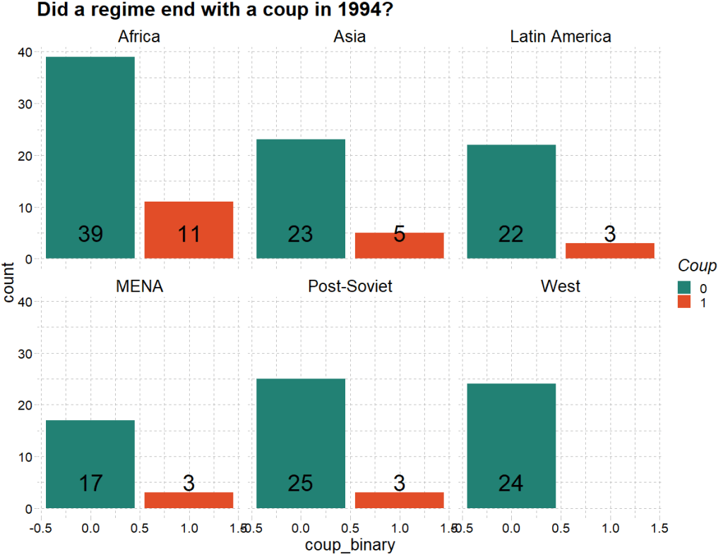

Okay, next on to the modelling.

With this new binary variable, we run a straightforward logistic regression in R.

To do this in R, we can run a generalised linear model and specify the family argument to be “binomial” :

summary(model_bin_1 <- glm(coup_binary ~ diagonal_accountability + military_control_score,
 family = "binomial", data = vdem_2) 

However some of the key information we want is not printed in the default R summary table.

This is where the jtools package comes in. It was created by Jacob Long from the University of South Carolina to help create simple summary tables that we can modify in the function. Click here to read the CRAN package PDF.

The summ() function can give us more information about the fit of the binomial model. This function also works with regular OLS lm() type models.

Set the vifs argument to TRUE for a multicollineary check.

summ(model_bin_1, vifs = TRUE)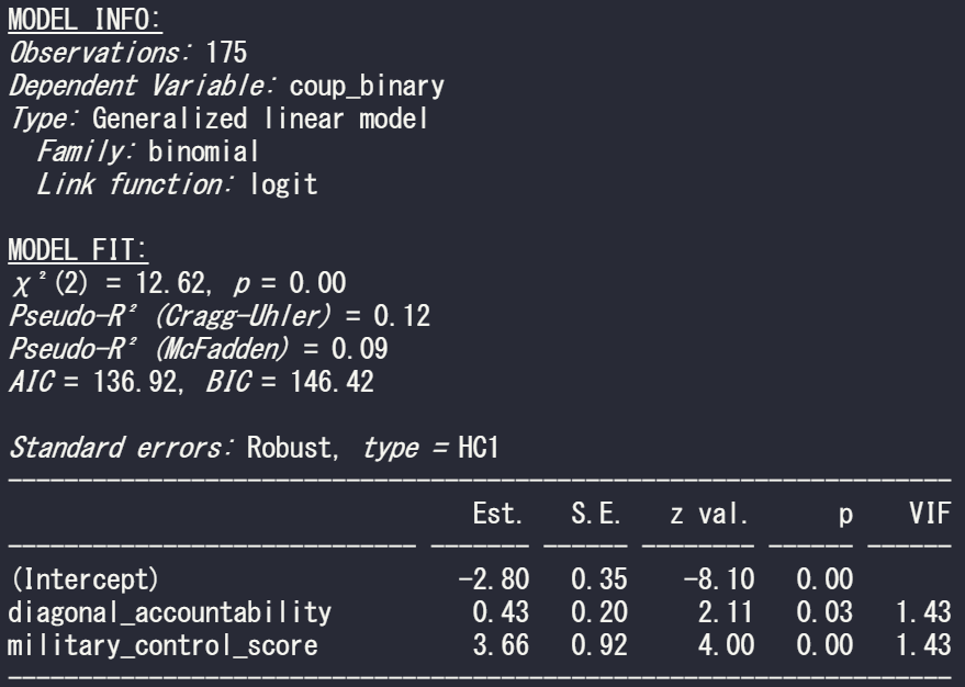

And we can see there is no problem with multicollinearity with the model; the VIF scores for the two independent variables in this model are well below 5.

Click here to read more about the Variance Inflation Factor and dealing with pesky multicollinearity.

In the above MODEL FIT section, we can see both the Cragg-Uhler (also known as Nagelkerke) and the McFadden Pseudo R² scores give a measure for the relative model fit. The Cragg-Uhler is just a modification of the Cox and Snell R².

There is no agreed equivalent to R² when we run a logistic regression (or other generalized linear models). These two Pseudo measures are just two of the many ways to calculate a Pseudo R² for logistic regression. Unfortunately, there is no broad consensus on which one is the best metric for a well-fitting model so we can only look at the trends of both scores relative to similar models. Compared to OLS R² , which has a general rule of thumb (e.g. an R² over 0.7 is considered a very good model), comparisons between Pseudo R² are restricted to the same measure within the same data set in order to be at all meaningful to us. However, a McFadden’s Pseudo R² ranging from 0.3 to 0.4 can loosely indicate a good model fit. So don’t be disheartened if your Pseudo scores seems to be always low.

If we add another continuous variable – judicial corruption score – we can see how this affects the overall fit of the model.

summary(model_bin_2 <- glm(coup_binary ~
     diagonal_accountability + 
     military_control_score + 
     judicial_corruption,
     family = "binomial", 
     data = vdem_2))

And run the summ() function like above:

summ(model_bin_2, vifs = TRUE)

The AIC of the second model is smaller, so this model is considered better. Additionally, both the Pseudo R² scores are larger! So we can say that the model with the additional judicial corruption variable is a better fitting model.

Click here to learn more about the AIC and choosing model variables with a stepwise algorithm function.

stargazer(model_bin, model_bin_2, type = "text")

One additional thing we can specify in the summ() function is the robust argument, which we can use to specify the type of standard errors that we want to correct for.

The assumption of homoskedasticity is does not need to be met in order to run a logistic regression. So I will run a “gaussian” general linear model (i.e. a linear model) to show the impact of changing the robust argument.

We suffer heteroskedasticity when the variance of errors in our model vary (i.e are not consistently random) across observations. It causes inefficient estimators and we cannot trust our p-values.

Click to learn more about checking for and correcting for heteroskedasticity in OLS.

We can set the robust argument to “HC1” This is the default standard error that Stata gives.

Set it to “HC3” to see the default standard error that we get with the sandwich package in R.

So run a simple regression to see the relationship between freedom from torture scale and the three independent variables in the model

summary(model_glm1 <- glm(freedom_torture ~ civil_lib + exec_bribe + judicial_corr, data = vdem90, family = "gaussian"))

Now I run the same summ() function but just change the robust argument:

First with no standard error correction. This means the standard errors are calculated with maximum likelihood estimators (MLE). The main problem with MLE is that is assumes normal distribution of the errors in the model.

summ(model_glm1, vifs = TRUE)

Next with the default STATA robust argument:

summ(model_glm1, vifs = TRUE, robust = "HC1")

And last with the default from R’s sandwich package:

summ(model_glm1, vifs = TRUE, robust = "HC3")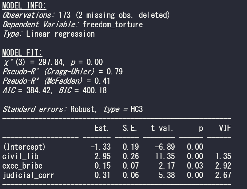

If we compare the standard errors in the three models, they are the highest (i.e. most conservative) with HC3 robust correction. Both robust arguments cause a 0.01 increase in the p-value but this is so small that it do not affect the eventual p-value significance level (both under 0.05!)