Add rectangular flags to maps in R

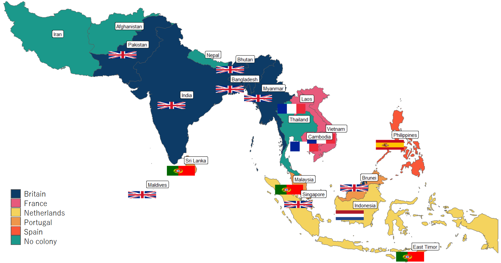
We will make a graph to map the different colonial histories of countries in South-East Asia!

Click here to add circular flags.

Packages we will need:

library(ggimage)
library(rnaturalearth)
library(countrycode)
library(ggthemes)
library(reshape2)

I use the COLDAT Colonial Dates Dataset by Bastien Becker (2020). We will only need the first nine columns in the dataset:

col_df <- data.frame(col_df[1:9])

Next we will need to turn the dataset from wide to long with the reshape2 package:

long_col <- melt(col_df, id.vars=c("country"), 
                 measure.vars = c("col.belgium","col.britain", "col.france", "col.germany", 
"col.italy", "col.netherlands",  "col.portugal", "col.spain"),
                 variable.name = "colony", 
                 value.name = "value")

We drop all the 0 values from the dataset:

long_col <- long_col[which(long_col$value == 1),]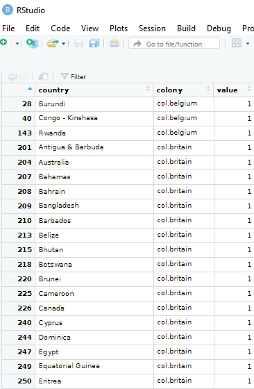

Next we use ne_countries() function from the rnaturalearth package to create the map!

map <- ne_countries(scale = "medium", returnclass = "sf")

Click here to read more about the rnaturalearth package.

Next we merge the two datasets together:

col_map <- merge(map, long_col, by.x = "iso_a3", by.y = "iso3", all.x = TRUE)

We can change the class and factors of the colony variable:

library(plyr)
col_map$colony_factor <- as.factor(col_map$colony)
col_map$colony_factor <- revalue(col_map$colony_factor, c("col.belgium"="Belgium", "col.britain" = "Britain",
 "col.france" = "France",
"col.germany" = "Germany",
 "col.italy" = "Italy",
 "col.netherlands" = "Netherlands", "col.portugal" = "Portugal",
 "col.spain" = "Spain",
 "No colony" = "No colony"))

Nearly there.

Next we will need to add the longitude and latitude of the countries. The data comes from the web and I can scrape the table with the rvest package

library(rvest)

coord <- read_html("https://developers.google.com/public-data/docs/canonical/countries_csv")

coord_tables <- coord %>% html_table(header = TRUE, fill = TRUE)

coord <- coord_tables[[1]]

col_map <- merge(col_map, coord, by.x= "iso_a2", by.y = "country", all.y = TRUE)

Click here to read more about the rvest package.

And we can make a vector with some hex colors for each of the European colonial countries.

my_palette <- c("#0d3b66","#e75a7c","#f4d35e","#ee964b","#f95738","#1b998b","#5d22aa","#85f5ff", "#19381F")

Next, to graph a map to look at colonialism in Asia, we can extract countries according to the subregion variable from the rnaturalearth package and graph.

asia_map <- col_map[which(col_map$subregion == "South-Eastern Asia" | col_map$subregion == "Southern Asia"),]

Click here to read more about the geom_flag function.

colony_asia_graph <- asia_map %>%
  ggplot() + geom_sf(aes(fill = colony_factor), 
                     position = "identity") +
  ggimage::geom_flag(aes(longitude-2, latitude-1, image = col_iso), size = 0.04) +
  geom_label(aes(longitude+1, latitude+1, label = factor(sovereignt))) +
  scale_fill_manual(values = my_palette)

And finally call the graph with the theme_map() from ggthemes package

References

Becker, B. (2020). Introducing COLDAT: The Colonial Dates Dataset.