With the European Social Survey (ESS), we will examine the different variables that are related to levels of trust in politicians across Europe in the latest round 9 (conducted in 2018).
Click here for Part 2.
Click here to learn about downloading ESS data into R with the essurvey package.
Packages we will need:
library(survey)
library(srvyr)
The survey package was created by Thomas Lumley, a professor from Auckland. The srvyr package is a wrapper packages that allows us to use survey functions with tidyverse.
Why do we need to add weights to the data when we analyse surveys?
When we import our survey data file, R will assume the data are independent of each other and will analyse this survey data as if it were collected using simple random sampling.
However, the reality is that almost no surveys use a simple random sample to collect data (the one exception being Iceland in ESS!)

Rather, survey institutions choose complex sampling designs to reduce the time and costs of ultimately getting responses from the public.
Their choice of sampling design can lead to different estimates and the standard errors of the sample they collect.
For example, the sampling weight may affect the sample estimate, and choice of stratification and/or clustering may mean (most likely underestimated) standard errors.
As a result, our analysis of the survey responses will be wrong and not representative to the population we want to understand. The most problematic result is that we would arrive at statistical significance, when in reality there is no significant relationship between our variables of interest.
Therefore it is essential we don’t skip this step of correcting to account for weighting / stratification / clustering and we can make our sample estimates and confidence intervals more reliable.
This table comes from round 8 of the ESS, carried out in 2016. Each of the 23 countries has an institution in charge of carrying out their own survey, but they must do so in a way that meets the ESS standard for scientifically sound survey design (See Table 1).

Sampling weights aim to capture and correct for the differing probabilities that a given individual will be selected and complete the ESS interview.
For example, the population of Lithuania is far smaller than the UK. So the probability of being selected to participate is higher for a random Lithuanian person than it is for a random British person.
Additionally, within each country, if the survey institution chooses households as a sampling element, rather than persons, this will mean that individuals living alone will have a higher probability of being chosen than people in households with many people.
Click here to read in detail the sampling process in each country from round 1 in 2002. For example, if we take my country – Ireland – we can see the many steps involved in the country’s three-stage probability sampling design.

The Primary Sampling Unit (PSU) is electoral districts. The institute then takes addresses from the Irish Electoral Register. From each electoral district, around 20 addresses are chosen (based on how spread out they are from each other). This is the second stage of clustering. Finally, one person is randomly chosen in each house to answer the survey, chosen as the person who will have the next birthday (third cluster stage).


Click here for more information about Design Effects (DEFF) and click here to read how ESS calculates design effects.
DEFF p refers to the design effect due to unequal selection probabilities (e.g. a person is more likely to be chosen to participate if they live alone)
DEFF c refers to the design effect due to clustering
According to Gabler et al. (1999), if we multiply these together, we get the overall design effect. The Irish design that was chosen means that the data’s variance is 1.6 times as large as you would expect with simple random sampling design. This 1.6 design effects figure can then help to decide the optimal sample size for the number of survey participants needed to ensure more accurate standard errors.

So, we can use the functions from the survey package to account for these different probabilities of selection and correct for the biases they can cause to our analysis.
In this example, we will look at demographic variables that are related to levels of trust in politicians. But there are hundreds of variables to choose from in the ESS data.
Click here for a list of all the variables in the European Social Survey and in which rounds they were asked. Not all questions are asked every year and there are a bunch of country-specific questions.

We can look at the last few columns in the data.frame for some of Ireland respondents (since we’ve already looked at the sampling design method above).
The dweight is the design weight and it is essentially the inverse of the probability that person would be included in the survey.
The pspwght is the post-stratification weight and it takes into account the probability of an individual being sampled to answer the survey AND ALSO other factors such as non-response error and sampling error. This post-stratificiation weight can be considered a more sophisticated weight as it contains more additional information about the realities survey design.
The pweight is the population size weight and it is the same for everyone in the Irish population.

When we are considering the appropriate weights, we must know the type of analysis we are carrying out. Different types of analyses require different combinations of weights. According to the ESS weighting documentation:
- when analysing data for one country alone – we only need the design weight or the poststratification weight.
- when comparing data from two or more countries but without reference to statistics that combine data from more than one country – we only need the design weight or the poststratification weight
- when comparing data of two or more countries and with reference to the average (or combined total) of those countries – we need BOTH design or post-stratification weight AND population size weights together.
- when combining different countries to describe a group of countries or a region, such as “EU accession countries” or “EU member states” = we need BOTH design or post-stratification weights AND population size weights.
ESS warn that their survey design was not created to make statistically accurate region-level analysis, so they say to carry out this type of analysis with an abundance of caution about the results.
ESS has a table in their documentation that summarises the types of weights that are suitable for different types of analysis:

Since we are comparing the countries, the optimal weight is a combination of post-stratification weights AND population weights together.
Click here to read Part 2 and run the regression on the ESS data with the survey package weighting design
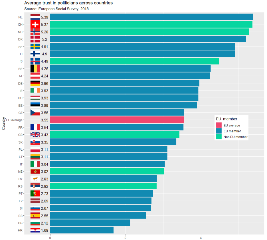
Below is the code I use to graph the differences in mean level of trust in politicians across the different countries.
library(ggimage) # to add flags
library(countrycode) # to add ISO country codes

# r_agg is the aggregated mean of political trust for each countries' respondents.

r_agg %>%
  dplyr::mutate(country, EU_member = ifelse(country == "BE" | country == "BG" | country == "CZ" | country == "DK" | country == "DE" | country == "EE" | country == "IE" | country == "EL" | country == "ES" | country == "FR" | country == "HR" | country == "IT" | country == "CY" | country == "LV" | country == "LT" | country == "LU" | country == "HU" | country == "MT" | country == "NL" | country == "AT" | country == "AT" | country == "PL" | country == "PT" | country == "RO" | country == "SI" | country == "SK" | country == "FI" | country == "SE","EU member", "Non EU member")) -> r_agg


r_agg %>%
  filter(EU_member == "EU member") %>%
  dplyr::summarize(eu_average = mean(mean_trust_pol))


r_agg$country_name <- countrycode(r_agg$country, "iso2c", "country.name")


#eu_average <- r_agg %>%
 # summarise_if(is.numeric, mean, na.rm = TRUE)


eu_avg <- data.frame(country = "EU average",
                     mean_trust_pol = 3.55,
                     EU_member =  "EU average",
                     country_name = "EU average")

r_agg <- rbind(r_agg, eu_avg)


my_palette <- c("EU average" = "#ef476f",
                "Non EU member" = "#06d6a0",
                "EU member" = "#118ab2")

r_agg <- r_agg %>%
  dplyr::mutate(ordered_country = fct_reorder(country, mean_trust_pol))


r_graph <- r_agg %>%
  ggplot(aes(x = ordered_country, y = mean_trust_pol, group = country, fill = EU_member)) +
  geom_col() +
  ggimage::geom_flag(aes(y = -0.4, image = country), size = 0.04) +
  geom_text(aes(y = -0.15 , label = mean_trust_pol)) +
  scale_fill_manual(values = my_palette) + coord_flip()

r_graph 
