Wrangling and graphing UN Secretaries-General data with R

Packages we will need:

library(tidyverse)
library(janitor)
library(rvest)
library(countrycode)
library(magrittr)
library(lubridate)
library(ggflags)
library(scales)

According to Urquhart (1995) in his article, “Selecting the World’s CEO”,

From the outset, the U.N. secretary
general has been an important part of the
institution, not only as its chief executive,
but as both symbol and guardian of the
original vision of the organization.
There, however, specific agreement has
ended. The United Nations, like any
important organization, needs strong and
independent leadership, but it is an inter-
governmental organization, and govern
ments have no intention of giving up
control of it. While the secretary-general
can be extraordinarily useful in times of
crisis, the office inevitably embodies
something more than international coop
eration, sometimes even an unwelcome
hint of supranationalism. Thus, the atti-
tude of governments toward the United
Nations’ chief and only elected official is
and has been necessarily ambivalent.

(Urquhart, 1995: 21)

So who are these World CEOs? We’ll examine more in this dataset.

First, we will scrape the data from the Wikipedia

sg_html <- read_html("https://en.wikipedia.org/wiki/Secretary-General_of_the_United_Nations")
sg_tables <- sg_html %>% html_table(header = TRUE, fill = TRUE)
sg <- sg_tables[[2]]

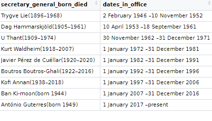
The table we scrape is a bit of a hot mess in this state …. but we can fix it

Donald Glover Pizza GIF - Find & Share on GIPHY

We can first use the clean_names() function from the janitor package

A quick way to clean up the table and keep only the rows with the names of the Secretaries-General is to use the distinct() function. Last we filter out the rows and select out the columns we don’t want.

sg %>% 
  clean_names() %>% 
  distinct(no, .keep_all = TRUE) %>% 
  filter(no != "–") %>% 
  select(!c(portrait, ref))-> sg_clean

Already we can see a much cleaner table. However, the next problem is that the names and their years of birth / death are in one cell.

Also the dates in office are combined together.

So we can use the separate() function from tidyr to make new variables for each piece of information.

First we will separate the name of the Secretary-General from their date of birth and death.

We supply the two new variable names to the into = argument.

We then use the regex code pattern [()] to indicate where we want to separate the character string into two separate columns. In this instance the regex pattern is for what is after the round brackets (

I want to remove the original cluttered varaible so remove = TRUE

sg_clean %<>% 
  separate(
    col = secretary_general_born_died,
    into = c("sec_gen", "born_died"),
    sep = '[()]',
    remove = TRUE)

We can repeat this step to create a separate born and died variable. This time the separator symbol is a hyphen And so we do not need regex pattern; we can just indicate a hyphen.

sg_clean %<>% 
  separate(
    col = born_died,
    into = c("born", "died"),
    sep = '–',
    remove = TRUE)

And I want to ignore the “present” variable, so I extract the numbers with the parse_number() function, converting things from characters to numbers

sg_clean %<>% 
  mutate(born = parse_number(born))

Last, we repeat with the dates in office. This is also easily seperated by indicating the hyphen.

sg_clean %<>% 
  separate(
    col = dates_in_office,
    into = c("start_office", "end_office"),
    sep = '–',
    remove = TRUE)

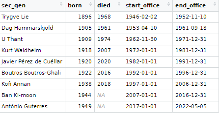
We convert the word “present” to the actual present date

sg_clean %<>% 
  mutate(end_office = ifelse(end_office == "present", "5 May 2022", end_office))

We use the lubridate dmy() function to convert the character strings to date class variables.

sg_clean %<>% 
  mutate(start_office = dmy(start_office),
         end_office = dmy(end_office))

We can calculate the length of time that each Secretary-General was in office with the difftime() function.

sg_clean %<>% 
  mutate(duration_days = difftime(end_office, start_office, units = "days"),
         duration_years = round(duration_days / 365, 2),
         duration_years = as.integer(duration_years))

Next we can compare the different durations and see which Secretary-General was longest or shortest in office.

sg_clean %>% 
  mutate(duration_days = difftime(end_office, start_office)) %>%  
  mutate(iso2 = tolower(countrycode::countrycode(country_of_origin, "country.name", "iso2c"))) %>% 
  ggplot(aes(x = forcats::fct_reorder(sec_gen, duration_days), y = duration_days)) + 
  geom_bar(aes(fill = un_regional_group), stat = "identity", width = 0.7) + 
  coord_flip() + bbplot::bbc_style() + 
  ggflags::geom_flag(aes(x = sec_gen, y = -100, country = iso2), size = 12) +
  scale_fill_manual(values = le_palette) +
  labs(title = "Longest serving UN Secretaries General",
       subtitle = ("Source: Wikipedia")) + 
  xlab("") + ylab("")

We can make a quick pie-chart to compare regions. We can see that Secretaries-General from the West have had the most time in office

sg_text <- sg_count %>% 
  arrange(desc(un_regional_group)) %>%
  mutate(prop = sum_days / sum(sg_count$sum_days) *100) %>%
  mutate(ypos = cumsum(prop)- 0.5*prop )

sg_text %>% 
  count(un_regional_group)

sg_text %>%
  mutate(region = case_when(un_regional_group == "Western European & others" ~ "Europe",
         un_regional_group == "Latin American& Caribbean" ~ "Latin America",
         un_regional_group == "Asia & Pacific" ~ "Asia", 
         TRUE ~ as.character(un_regional_group))) %>% 
  ggplot(aes(x = "", y = prop, fill = region)) +
  geom_bar(stat = "identity", width = 1) +
  geom_text(aes(y = ypos + 1, label = round(prop, 0)), color = "white", size = 15) +
  coord_polar("y", start = 0) +
  theme_void() +
  ggtitle("Length of Secretaries General in office across regions") + 
  scale_fill_manual(values = le_palette) + 
  theme(legend.title = element_blank(),
        legend.text = element_text(size = 20), 
        plot.title = element_text(size = 30))

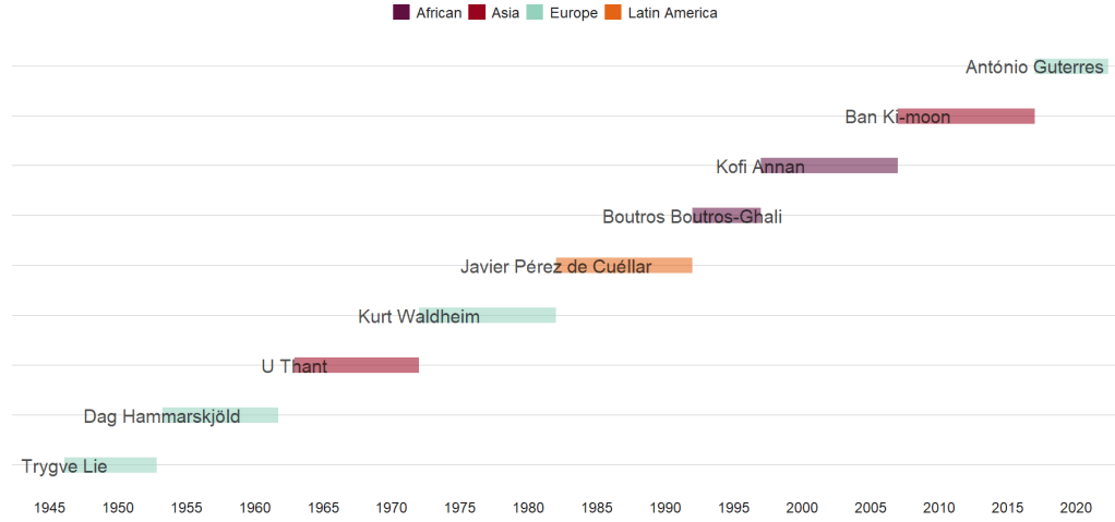
We can create a Gantt-like chart to track the timeline for the different men (all men!)

Click here to read more about timelines in R

Make a timeline graph with dates in ggplot2

sg_clean %>% 
  mutate(region = case_when(un_regional_group == "Western European & others" ~ "Europe",un_regional_group == "Latin American& Caribbean" ~ "Latin America",un_regional_group == "Asia & Pacific" ~ "Asia", TRUE ~ as.character(un_regional_group))) %>%
  ggplot(aes(x = as.Date(start_office), 
             y = no, 
             color = region)) +
  geom_segment(aes(xend = as.Date(end_office), 
                   yend = no, alpha = 0.9,
                   color = region), size = 9)  +
  geom_text(aes(label = sec_gen), 
            color = "black", 
            alpha = 0.7,
            size = 8, show.legend = FALSE) +
  bbplot::bbc_style() +
  scale_color_manual(values = le_palette) + 
  scale_x_date(breaks = scales::breaks_pretty(15))

References

Urquhart, B. (1995). Selecting the world’s CEO: Remembering the Secretaries-General. Foreign Affairs, 21-26.