How to graph Locally Weighted Scatterplot Smoothing (LOESS) in R

The loess method in ggplot2 fits a smoothing line to our data.

We can do this with the method = "loess" in the geom_smooth() layer.

LOESS stands “Locally Weighted Scatterplot Smoothing.” (I am not sure why it is not called LOWESS … ?)

The loess line can help show non-linear relationships in the scatterplot data, while taking care of stopping the over-influence of outliers.

Loess gives more weight to nearby data points and less weight to distant ones. This means that nearby points have a greater influence on the squiggly-ness of the line.

The degree of smoothing is controlled by the span parameter in the geom_smooth() layer.

When we set the span, we can choose how many nearby data points are considered when estimating the local regression line.

A smaller span (e.g. span = 0.5) results in more local (flexible) smoothing, while a larger span (e.g. span = 1.5) produces more global (smooth) smoothing.

We will take the variables from the Varieties of Democracy dataset and plot the relationship between oil produciton and media freedoms across different regions.

df %>% 
  ggplot(aes(x = log_avg_oil,
             y = avg_media)) +
  geom_point(size = 6, alpha = 0.5) + 
  geom_smooth(aes(color = region), 
              method = "loess", 
              span = 2,
              se = FALSE,
              size = 3,
              alpha = 0.6) + 
  facet_wrap(~region) + 
  labs(title = "Oil and Media Corruption", subtitle = "VDEM",
       x = "Average Oil logged",
       y = "Average Media Freedom") +
  scale_color_manual(values = my_pal) + 
  my_theme()

If we change the span to 0.5, we get the following graph:

              span = 0.5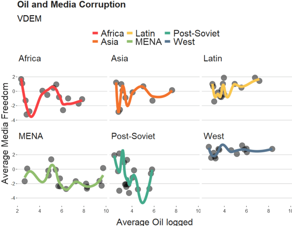

When examining the connection between oil production and media freedoms across various regions, there are many ways to draw the line.

If we think the relationship is linear, it is no problem to add method = "lm" to the graph.

However, if outliers might overly distort the linear relationship, method = "rlm" (robust linear model” can help to take away the power from these outliers.

Linear and robust linear models (lm and rlm) can also accommodate parametric non-linear relationships, such as quadratic or cubic, when used with a proper formula specification.

For example, “geom_smooth(method=’lm’, formula = y ~ x + I(x^2))” can be used for estimating a quadratic relationship using lm.

If the outcome variable is binary (such as “is democracy” versus “is not democracy” or “is oil producing” versus “is not oil producing”) we can use method = “glm” (which is generalised linear model). It models the log odds of a oil producing as a linear function of a predictor variable, like age.

If the relationship between age and log odds is non-linear, the gam method is preferred over glm. Both glm and gam can handle outcome variables with more than two categories, count variables, and other complexities.