How to run cross-validation of decision-tree models with xgboost in R (PART 4 Tidymodels series)

In this blog post, we will cross-validate different boosted tree models and find the one with best root mean square error (RMSE).

Specifically, part 2 goes into more detail about RMSE as a way to choose the best model

Click here to read part 1, part 2 or part 3 of this series on tidymodel package stuff.

Packages we will need:

library(tidymodels)
library(tidyverse)

Our resampling method will be 10-fold cross-validation.

Click here to watch a Youtube explainer by StatQuest on the fundamentals of cross validation. StatQuest is the cat’s pyjamas.

We can use the vfold_cv() function to create a set of “V-fold” cross-validation with 11 splits.

My favorite number is 11 so I’ll set that as the seed too.

set.seed(11) 
cross_folds <- vfold_cv(vdem_1990_2019, v = 11)

We put our formula into the recipe function and run the pre-processing steps: in this instance, we are just normalizing the variables.

my_recipe <- recipe(judic_corruption ~ freedom_religion + polarization, 
data = vdem_1990_2019) %>%
step_normalize(all_predictors(), -all_outcomes())

Here, we will initially define a boost_tree() model without setting any hyperparameters.

This is our baseline model with defaults.

With the vfolds, we be tuning them and choosing the best parameters.

For us, our mode is “regression” (not categorical “classification”)

my_tree <- boost_tree(
mode = "regression",
engine = "xgboost") %>%
set_engine("xgboost") %>%
set_mode("regression")

Next we will set up a grid to explore a range of hyperparameters.

my_grid <- grid_latin_hypercube(
trees(range = c(500, 1500)),
tree_depth(range = c(3, 10)),
learn_rate(range = c(0.01, 0.1)),
size = 20)

We use the grid_latin_hypercube() function from the dials package in R is used to generate a sampling grid for tuning hyperparameters using a Latin hypercube sampling method.

Latin hypercube sampling (LHS) is a way to generate a sample of plausible, semi-random collections of parameter values from a distribution.

This method is used to ensure that each parameter is uniformly sampled across its range of values. LHS is systematic and stratified, but within each stratum, it employs randomness.

Source: https://www.youtube.com/watch?app=desktop&v=Evua529dAgc

Inside the grid_latin_hypercube() function,we can set the ranges for the model parameters,

trees(range = c(500, 1500))

This parameter specifies the number of trees in the model

We can set a sampling range from 500 to 1500 trees.

tree_depth(range = c(3, 10))

This defines the maximum depth of each tree

We set values ranging from 3 to 10.

learn_rate(range = c(0.01, 0.1))

This parameter controls the learning rate, or the step size at each iteration while moving toward a minimum of a loss function.

It’s specified to vary between 0.01 and 0.1.

size = 20

We want the Latin Hypercube Sampling to generate 20 unique combinations of the specified parameters. Each of these combinations will be used to train a model, allowing for a systematic exploration of how different parameter settings impact model performance.

> my_grid

# A tibble: 20 × 3
   trees tree_depth learn_rate
   <int>      <int>      <dbl>
 1   803          7       1.03
 2   981          7       1.18
 3   862          6       1.09
 4  1185          9       1.06
 5   763          8       1.13
 6   593          4       1.11
 7   524          7       1.22
 8   743          3       1.17
 9  1347          5       1.07
10  1010          5       1.15
11   677          3       1.25
12  1482          5       1.05
13  1446          8       1.12
14   917          4       1.23
15  1296          6       1.04
16  1391          8       1.23
17  1106          9       1.18
18  1203          5       1.14
19   606         10       1.20
20  1088          9       1.10

So next, we will combine our recipe, model specification, and resampling method in a workflow, and use tune_grid() to find the best hyperparameters based on RMSE.

my_workflow <- workflow() %>%
add_recipe(my_recipe) %>%
add_model(my_tree)

The tune_grid() function does the hyperparameter tuning. We will make different combinations of hyperparameters specified in grid using cross-validation.

tuning_results <- my_workflow %>%
tune_grid(
resamples = cv_folds,
grid = my_grid,
metrics = metric_set(rmse))
# Tuning results
# 10-fold cross-validation 
# A tibble: 10 × 4
   splits             id     .metrics         .notes          
   <list>             <chr>  <list>           <list>          
 1 <split [3200/356]> Fold01 <tibble [1 × 4]> <tibble [0 × 3]>
 2 <split [3200/356]> Fold02 <tibble [1 × 4]> <tibble [0 × 3]>
 3 <split [3200/356]> Fold03 <tibble [1 × 4]> <tibble [0 × 3]>
 4 <split [3200/356]> Fold04 <tibble [1 × 4]> <tibble [0 × 3]>
 5 <split [3200/356]> Fold05 <tibble [1 × 4]> <tibble [0 × 3]>
 6 <split [3200/356]> Fold06 <tibble [1 × 4]> <tibble [0 × 3]>
 7 <split [3201/355]> Fold07 <tibble [1 × 4]> <tibble [0 × 3]>
 8 <split [3201/355]> Fold08 <tibble [1 × 4]> <tibble [0 × 3]>
 9 <split [3201/355]> Fold09 <tibble [1 × 4]> <tibble [0 × 3]>
10 <split [3201/355]> Fold10 <tibble [1 × 4]> <tibble [0 × 3]>

After tuning, we can extract and examine the best models.

show_best(tuning_results, metric = "rmse")
  trees tree_depth learn_rate .metric .estimator  mean     n std_err .config              
  <int>      <int>      <dbl> <chr>   <chr>      <dbl> <int>   <dbl> <chr>                
1   593          4       1.11 rmse    standard   0.496    10  0.0189 Preprocessor1_Model03
2   677          3       1.25 rmse    standard   0.500    10  0.0216 Preprocessor1_Model02
3  1296          6       1.04 rmse    standard   0.501    10  0.0238 Preprocessor1_Model09
4  1010          5       1.15 rmse    standard   0.501    10  0.0282 Preprocessor1_Model08
5  1482          5       1.05 rmse    standard   0.502    10  0.0210 Preprocessor1_Model05

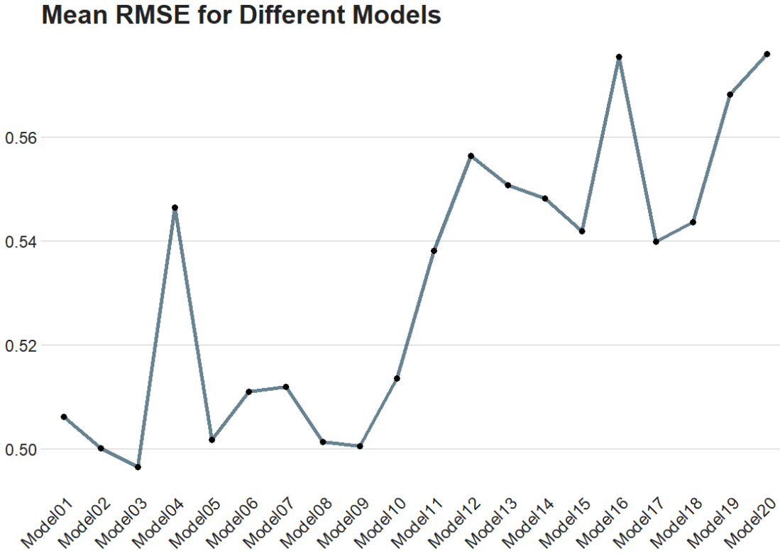
The best model is model number 3!

The Fresh Prince Of Bel Air Reaction GIF - Find & Share on GIPHY

Finally, we can plot it out.

We use collect_metrics() to pull out the RMSE and other metrics from our samples.

It automatically aggregates the results across all resampling iterations for each unique combination of model hyperparameters, providing mean performance metrics (e.g., mean accuracy, mean RMSE) and their standard errors.

rmse_results <- tuning_results %>%
collect_metrics() %>%
filter(.metric == "rmse")
rmse_results %>%
mutate(.config = str_replace(.config, "^Preprocessor1_", "")) %>%
ggplot(aes(x = .config, y = mean)) +
geom_line(aes(group = 1), color = "#023047", size = 2, alpha = 0.6) +
geom_point(size = 3) +
bbplot::bbc_style() +
labs(title = "Mean RMSE for Different Models") +
theme(axis.text.x = element_text(angle = 45, hjust = 1))

Comparing North and South Korean UN votes at the General Assembly with unvotes package

Packages we will use

Llibrary(unvotes)
library(lubridate)
library(tidyverse)
library(magrittr)
library(bbplot)
library(waffle)
library(stringr)
library(wordcloud)
library(waffle)
library(wesanderson)

Last September 17th 2021 marked the 30th anniversary of the entry of North Korea and South Korea into full membership in the United Nations. Prior to this, they were only afforded observer status.

keia.org

The Two Koreas Mark 30 Years of UN Membership: The Road to Membership

Let’s look at the types of voting that both countries have done in the General Assembly since 1991.

First we can download the different types of UN votes from the unvotes package

un_votes <- unvotes::un_roll_calls

un_votes_issues <- unvotes::un_roll_call_issues

unvotes::un_votes -> country_votes 

Join them all together and filter out any country that does not have the word “Korea” in its name.

un_votes %>% 
  inner_join(un_votes_issues, by = "rcid") %>% 
  inner_join(country_votes, by = "rcid") %>% 
  mutate(year = format(date, format = "%Y")) %>%
  filter(grepl("Korea", country)) -> korea_un

First we can make a wordcloud of all the different votes for which they voted YES. Is there a discernable difference in the types of votes that each country supported?

First, download the stop words that we can remove (such as the, and, if)

data("stop_words") 

Then I will make a North Korean dataframe of all the votes for which this country voted YES. I remove some of the messy formatting with the gsub argument and count the occurence of each word. I get rid of a few of the procedural words that are more related to the technical wording of the resolutions, rather than related to the tpoic of the vote.

nk_yes_votes <- korea_un %>% 
  filter(country == "North Korea") %>% 
  filter(vote == "yes") %>%  
  select(descr, year) %>% 
  mutate(decade = substr(year, 1, 3)) %>% 
  mutate(decade = paste0(decade, "0s")) %>% 
  # group_by(decade) %>% 
  unnest_tokens(word, descr) %>% 
  mutate(word = gsub(" ", "", word)) %>% 
  mutate(word = gsub('_', '', word)) %>% 
  count(word, sort = TRUE) %>% 
  ungroup() %>% 
  anti_join(stop_words)  %>% 
  mutate(word = case_when(grepl("palestin", word) ~ "Palestine", 
                          grepl("nucl", word) ~ "nuclear",
                          TRUE ~ as.character(word)))  %>%
  filter(word != "resolution") %>% 
  filter(word != "assembly") %>% 
  filter(word != "draft") %>% 
  filter(word != "committee") %>% 
  filter(word != "requested") %>% 
  filter(word != "report") %>% 
  filter(word != "practices") %>% 
  filter(word != "affecting") %>% 
  filter(word != "follow") %>% 
  filter(word != "acting") %>% 
  filter(word != "adopted") 

Next, we count the number of each word


nk_yes_votes %<>% 
  count(word) %>% 
  arrange(desc(n))

We want to also remove the numbers

nums <- nk_yes_votes %>% filter(str_detect(word, "^[0-9]")) %>% select(word) %>% unique()

And remove the stop words

nk_yes_votes %<>%
  anti_join(nums, by = "word")

Choose some nice colours

my_colors <- c("#0450b4", "#046dc8", "#1184a7","#15a2a2", "#6fb1a0", 
               "#b4418e", "#d94a8c", "#ea515f", "#fe7434", "#fea802")

And lastly, plot the wordcloud with the top 50 words

wordcloud(nk_yes_votes$word, 
   nk_yes_votes$n, 
   random.order = FALSE, 
   max.words = 50, 
   colors = my_colors)

If we repeat the above code with South Korea:

There doesn’t seem to be a huge difference. But this is not a very scientfic approach; I just like the look of them!

Next we will compare the two countries how many votes they voted yes, no or abstained from…

korea_un %>% 
  group_by(country, vote) %>% 
  count() %>% 
  mutate(count_ten = n /25) %>% 
  ungroup() %>% 
  ggplot(aes(fill = vote, values = count_ten)) +
  geom_waffle(color = "white",
              size = 2.5,
              n_rows = 10,
              flip = TRUE) +
  facet_wrap(~country) + bbplot::bbc_style() +
  scale_fill_manual(values = wesanderson::wes_palette("Darjeeling1"))

AND some tweaking with Canva

Next we can look more in detail at the votes that they countries abstained from voting in.

We can use the tidytext function that reorders the geom_bar in each country. You can read the blog of Julie Silge to learn more about the functions, it is a bit tricky but it fixes the problem of randomly ordered bars across facets.

https://juliasilge.com/blog/reorder-within/

korea_un %>%
  filter(vote == "abstain") %>% 
  mutate(issue = case_when(issue == "Nuclear weapons and nuclear material" ~ "Nukes",
issue == "Arms control and disarmament" ~ "Arms",
issue == "Palestinian conflict" ~ "Palestine",
TRUE ~ as.character(issue))) %>% 
  select(country, issue, year) %>% 
  group_by(issue, country) %>% 
  count() %>% 
  ungroup() %>% 
  group_by(country) %>% 
  mutate(country = as.factor(country),
         issue = reorder_within(issue, n, country)) %>%
  ggplot(aes(x = reorder(issue, n), y = n)) + 
  geom_bar(stat = "identity", width = 0.7, aes(fill = country)) + 
  labs(title = "Abstaining UN General Assembly Votes by issues",
       subtitle = ("Since 1950s"),
       caption = "         Source: unvotes ") +
  xlab("") + 
  ylab("") +
  facet_wrap(~country, scales = "free_y") +
  scale_x_reordered() +
  coord_flip() + 
  expand_limits(y = 65) + 
  ggthemes::theme_pander() + 
  scale_fill_manual(values = sample(my_colors)) + 
 theme(plot.background = element_rect(color = "#f5f9fc"),
        panel.grid = element_line(colour = "#f5f9fc"),
        # axis.title.x = element_blank(),
        # axis.text.x = element_blank(),
        axis.text.y = element_text(color = "#000500", size = 16),
       legend.position = "none",
        # axis.title.y = element_blank(),
        axis.ticks.x = element_blank(),
        text = element_text(family = "Gadugi"),
        plot.title = element_text(size = 28, color = "#000500"),
        plot.subtitle = element_text(size = 20, color = "#484e4c"),
        plot.caption = element_text(size = 20, color = "#484e4c"))

South Korea was far more likely to abstain from votes that North Korea on all issues

Next we can simply plot out the Human Rights votes that each country voted to support. Even though South Korea has far higher human rights scores, North Korea votes in support of more votes on this topic.

korea_un %>% 
  filter(year < 2019) %>% 
  filter(issue == "Human rights") %>% 
  filter(vote == "yes") %>% 
  group_by(country, year) %>% 
  count() %>% 
  ggplot(aes(x = year, y = n, group = country, color = country)) + 
  geom_line(size = 2) + 
  geom_point(aes(color = country), fill = "white", shape = 21, size = 3, stroke = 2.5) +
  scale_x_discrete(breaks = round(seq(min(korea_un$year), max(korea_un$year), by = 10),1)) +
  scale_y_continuous(expand = c(0, 0), limits = c(0, 22)) + 
  bbplot::bbc_style() + facet_wrap(~country) + 
  theme(legend.position = "none") + 
  scale_color_manual(values = sample(my_colors)) + 
  labs(title = "Human Rights UN General Assembly Yes Votes ",
       subtitle = ("Since 1990s"),
       caption = "         Source: unvotes ")

All together:

Grouping, counting words and making wordclouds

library(tidytext)
library(wordcloud)
library(knitr)
library(kableExtra)

How to make wordclouds in R!

First, download stop words (such as and, the, of) to filter out of the dataset

data("stop_words")

Then we will will unnest tokens and count the occurences of each word in each decade.

tokens <- democracy_aid %>%
  select(description, year) %>% 
  mutate(decade = substr(year, 1, 3)) %>% 
  mutate(decade = paste0(decade, "0s")) %>% 
  group_by(decade) %>% 
  unnest_tokens(word, activity_description) %>% 
  count(word, sort = TRUE) %>% 
  ungroup() %>% 
  anti_join(stop_words) 

nums <- tokens %>% filter(str_detect(word, "^[0-9]")) %>% select(word) %>% unique()

tokens %<>%
  anti_join(nums, by = "word") 

And with the kable() function we can make a HTML table that I copy and paste to this blog. Below I rewrite the HTML to change the headings

tokens %>% 
    group_by(decade) %>% 
    top_n(n = 10,
          wt = n)  %>%
    arrange(decade, desc(n)) %>%
    arrange(desc(n)) %>%
    knitr::kable("html")
decade word n
2010s rights 4541
2010s local 3981
2010s youth 3778
2010s promote 3679
2010s democratic 3618
2010s public 3444
2010s national 3060
2010s political 3020
2010s human 3009
2010s organization 2711
2000s rights 2548
2000s human 1745
2000s local 1544
2000s conduct 1381
2000s political 1257
2000s training 1217
2000s promote 1142
2000s public 1121
2000s democratic 1071
2000s national 988

Create a vector of colors:

my_colors <- c("#0450b4", "#046dc8", "#1184a7","#15a2a2", "#6fb1a0", 
               "#b4418e", "#d94a8c", "#ea515f", "#fe7434", "#fea802")
Always Sunny Reaction GIF - Find & Share on GIPHY
tokens %<>% 
  mutate(word = ifelse(grepl("democr", word), "democracy", 
                ifelse(grepl("politi", word), "politics", 
                ifelse(grepl("institut", word), "institution", 
                ifelse(grepl("govern", word), "government", 
                ifelse(grepl("organiz", word), "organization", 
                ifelse(grepl("elect", word), "election", word))))))) 

wordcloud(tokens$word, tokens$n, random.order = FALSE, max.words = 50, colors = my_colors)
2010s Decade Word Count
2010s rights 4541
2010s local 3981
2010s youth 3778
2010s promote 3679
2010s democratic 3618
2010s public 3444
2010s national 3060
2010s political 3020
2010s human 3009
2010s organization 2711
2000s Decade Word Count
2000s rights 2548
2000s human 1745
2000s local 1544
2000s conduct 1381
2000s political 1257
2000s training 1217
2000s promote 1142
2000s public 1121
2000s democratic 1071
2000s national 988

And if we compare civic versus politically-oriented aid, we can see that more money goes towards projects that have political or electoral aims rather than civic or civil society education goals

tokens %>% 
  group_by(year) %>% 
  top_n(n = 20,
        wt = n) %>% 
  mutate(word = case_when(word == "party" ~ "political",
                          word == "parties" ~ "political",
                          word == "election" ~ "political",
                          word == "electoral" ~ "political",
                          word == "civil" ~ "civic", 
                          word == "civic" ~ "civic",
                          word == "social" ~ "civic",
                          word == "education" ~ "civic",
                          word == "society" ~ "civic", 
                          TRUE ~ as.character(word))) %>% 
  filter(word == "political" | word == "civic") %>% 
  ggplot(aes(x = year, y = n, group = word)) + 
  geom_line(aes(color = word ), size = 2.5,alpha = 0.6)  +
  geom_point(aes(color = word ), fill = "white", 
             shape = 21, size = 3, stroke = 2) +
  bbplot::bbc_style() + 
  scale_x_discrete(limits = c(2001:2019)) +
  theme(axis.text.x= element_text(size = 15,
                                  angle = 45)) +
  scale_color_discrete(name = "Aid type", labels = c("Civic grants", "Political grants"))