Comparing North and South Korean UN votes at the General Assembly with unvotes package

Packages we will use

Llibrary(unvotes)
library(lubridate)
library(tidyverse)
library(magrittr)
library(bbplot)
library(waffle)
library(stringr)
library(wordcloud)
library(waffle)
library(wesanderson)

Last September 17^th 2021 marked the 30^th anniversary of the entry of North Korea and South Korea into full membership in the United Nations. Prior to this, they were only afforded observer status.

keia.org
The Two Koreas Mark 30 Years of UN Membership: The Road to Membership

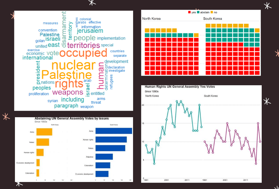
Let’s look at the types of voting that both countries have done in the General Assembly since 1991.

First we can download the different types of UN votes from the unvotes package

un_votes <- unvotes::un_roll_calls

un_votes_issues <- unvotes::un_roll_call_issues

unvotes::un_votes -> country_votes

Join them all together and filter out any country that does not have the word “Korea” in its name.

un_votes %>% 
  inner_join(un_votes_issues, by = "rcid") %>% 
  inner_join(country_votes, by = "rcid") %>% 
  mutate(year = format(date, format = "%Y")) %>%
  filter(grepl("Korea", country)) -> korea_un

First we can make a wordcloud of all the different votes for which they voted YES. Is there a discernable difference in the types of votes that each country supported?

First, download the stop words that we can remove (such as the, and, if)

data("stop_words")

Then I will make a North Korean dataframe of all the votes for which this country voted YES. I remove some of the messy formatting with the gsub argument and count the occurence of each word. I get rid of a few of the procedural words that are more related to the technical wording of the resolutions, rather than related to the tpoic of the vote.

nk_yes_votes <- korea_un %>% 
  filter(country == "North Korea") %>% 
  filter(vote == "yes") %>%  
  select(descr, year) %>% 
  mutate(decade = substr(year, 1, 3)) %>% 
  mutate(decade = paste0(decade, "0s")) %>% 
  # group_by(decade) %>% 
  unnest_tokens(word, descr) %>% 
  mutate(word = gsub(" ", "", word)) %>% 
  mutate(word = gsub('_', '', word)) %>% 
  count(word, sort = TRUE) %>% 
  ungroup() %>% 
  anti_join(stop_words)  %>% 
  mutate(word = case_when(grepl("palestin", word) ~ "Palestine", 
                          grepl("nucl", word) ~ "nuclear",
                          TRUE ~ as.character(word)))  %>%
  filter(word != "resolution") %>% 
  filter(word != "assembly") %>% 
  filter(word != "draft") %>% 
  filter(word != "committee") %>% 
  filter(word != "requested") %>% 
  filter(word != "report") %>% 
  filter(word != "practices") %>% 
  filter(word != "affecting") %>% 
  filter(word != "follow") %>% 
  filter(word != "acting") %>% 
  filter(word != "adopted")

Next, we count the number of each word


nk_yes_votes %<>% 
  count(word) %>% 
  arrange(desc(n))

We want to also remove the numbers

nums <- nk_yes_votes %>% filter(str_detect(word, "^[0-9]")) %>% select(word) %>% unique()

And remove the stop words

nk_yes_votes %<>%
  anti_join(nums, by = "word")

Choose some nice colours

my_colors <- c("#0450b4", "#046dc8", "#1184a7","#15a2a2", "#6fb1a0", 
               "#b4418e", "#d94a8c", "#ea515f", "#fe7434", "#fea802")

And lastly, plot the wordcloud with the top 50 words

wordcloud(nk_yes_votes$word, 
   nk_yes_votes$n, 
   random.order = FALSE, 
   max.words = 50, 
   colors = my_colors)

If we repeat the above code with South Korea:

There doesn’t seem to be a huge difference. But this is not a very scientfic approach; I just like the look of them!

Next we will compare the two countries how many votes they voted yes, no or abstained from…

korea_un %>% 
  group_by(country, vote) %>% 
  count() %>% 
  mutate(count_ten = n /25) %>% 
  ungroup() %>% 
  ggplot(aes(fill = vote, values = count_ten)) +
  geom_waffle(color = "white",
              size = 2.5,
              n_rows = 10,
              flip = TRUE) +
  facet_wrap(~country) + bbplot::bbc_style() +
  scale_fill_manual(values = wesanderson::wes_palette("Darjeeling1"))

Next we can look more in detail at the votes that they countries abstained from voting in.

We can use the tidytext function that reorders the geom_bar in each country. You can read the blog of Julie Silge to learn more about the functions, it is a bit tricky but it fixes the problem of randomly ordered bars across facets.

https://juliasilge.com/blog/reorder-within/

korea_un %>%
  filter(vote == "abstain") %>% 
  mutate(issue = case_when(issue == "Nuclear weapons and nuclear material" ~ "Nukes",
issue == "Arms control and disarmament" ~ "Arms",
issue == "Palestinian conflict" ~ "Palestine",
TRUE ~ as.character(issue))) %>% 
  select(country, issue, year) %>% 
  group_by(issue, country) %>% 
  count() %>% 
  ungroup() %>% 
  group_by(country) %>% 
  mutate(country = as.factor(country),
         issue = reorder_within(issue, n, country)) %>%
  ggplot(aes(x = reorder(issue, n), y = n)) + 
  geom_bar(stat = "identity", width = 0.7, aes(fill = country)) + 
  labs(title = "Abstaining UN General Assembly Votes by issues",
       subtitle = ("Since 1950s"),
       caption = "         Source: unvotes ") +
  xlab("") + 
  ylab("") +
  facet_wrap(~country, scales = "free_y") +
  scale_x_reordered() +
  coord_flip() + 
  expand_limits(y = 65) + 
  ggthemes::theme_pander() + 
  scale_fill_manual(values = sample(my_colors)) + 
 theme(plot.background = element_rect(color = "#f5f9fc"),
        panel.grid = element_line(colour = "#f5f9fc"),
        # axis.title.x = element_blank(),
        # axis.text.x = element_blank(),
        axis.text.y = element_text(color = "#000500", size = 16),
       legend.position = "none",
        # axis.title.y = element_blank(),
        axis.ticks.x = element_blank(),
        text = element_text(family = "Gadugi"),
        plot.title = element_text(size = 28, color = "#000500"),
        plot.subtitle = element_text(size = 20, color = "#484e4c"),
        plot.caption = element_text(size = 20, color = "#484e4c"))

South Korea was far more likely to abstain from votes that North Korea on all issues

Next we can simply plot out the Human Rights votes that each country voted to support. Even though South Korea has far higher human rights scores, North Korea votes in support of more votes on this topic.

korea_un %>% 
  filter(year < 2019) %>% 
  filter(issue == "Human rights") %>% 
  filter(vote == "yes") %>% 
  group_by(country, year) %>% 
  count() %>% 
  ggplot(aes(x = year, y = n, group = country, color = country)) + 
  geom_line(size = 2) + 
  geom_point(aes(color = country), fill = "white", shape = 21, size = 3, stroke = 2.5) +
  scale_x_discrete(breaks = round(seq(min(korea_un$year), max(korea_un$year), by = 10),1)) +
  scale_y_continuous(expand = c(0, 0), limits = c(0, 22)) + 
  bbplot::bbc_style() + facet_wrap(~country) + 
  theme(legend.position = "none") + 
  scale_color_manual(values = sample(my_colors)) + 
  labs(title = "Human Rights UN General Assembly Yes Votes ",
       subtitle = ("Since 1990s"),
       caption = "         Source: unvotes ")