Running a regression model with too many variables – especially irrelevant ones – will lead to a needlessly complex model. Stepwise can help to choose the best variables to add.

Packages you need:

library(olsrr)
library(MASS)
library(stargazer)

First, choose a model and throw every variable you think has an impact on your dependent variable!

I hear the voice of my undergrad professor in my ear: ” DO NOT go for the “throw spaghetti at the wall and just see what STICKS” approach. A cardinal sin.

We must choose variables because we have some theoretical rationale for any potential relationship. Or else we could end up stumbling on spurious relationships.

Like the one between Nick Cage movies and incidence of pool drowning.

However …

… beyond just using our sound theoretical understanding of the complex phenomena we study in order to choose our model variables …

… one additional way to supplement and gauge which variables add to – or more importantly omit from – the model is to choose the one with the smallest amount of error.

We can operationalise this as the model with the lowest Akaike information criterion (AIC).

AIC is an estimator of in-sample prediction error and is similar to the adjusted R-squared measures we see in our regression output summaries.

It effectively penalises us for adding more variables to the model.

Lower scores can indicate a more parsimonious model, relative to a model fit with a higher AIC. It can therefore give an indication of the relative quality of statistical models for a given set of data.

As a caveat, we can only compare AIC scores with models that are fit to explain variance of the same dependent / response variable.

data(mtcars)
car_model <- lm(mpg ~., data = mtcars) %>% stargazer

Very many variables and not many stars.

With our model, we can now feed it into the stepwise function. Hopefully, we can remove variables that are not contributing to the model!

For the direction argument, you can choose between backward and forward stepwise selection,

• Forward steps: start the model with no predictors, just one intercept and search through all the single-variable models, adding variables, until we find the the best one (the one that results in the lowest residual sum of squares)

• Backward steps: we start stepwise with all the predictors and removes variable with the least statistically significant (the largest p-value) one by one until we find the lost AIC.

Backward stepwise is generally better because starting with the full model has the advantage of considering the effects of all variables simultaneously.

Unlike backward elimination, forward stepwise selection is more suitable in settings where the number of variables is bigger than the sample size.

So tldr: unless the number of candidate variables is greater than the sample size (such as dealing with genes), using a backward stepwise approach is default choice.

You can also choose direction = "both":

step_car <- stepAIC(car_model, trace = TRUE, direction= "both")

If you add the trace = TRUE, R prints out all the steps.

I’ll show the last step to show you the output.

The goal is to have the combination of variables that has the lowest AIC or lowest residual sum of squares (RSS).

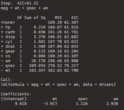
BThe best model, based on the lowest AIC, includes the predictors wt (weight), qsec (quarter-mile time), and am (automatic/manual transmission). The formula is mpg ~ wt + qsec + am.

If we dropped the wt variable, the AIC would shoot up 82.79, so we won’t do that.

Model Comparison:

The initial model (null model) has an AIC of 61.31.
Each row in the table corresponds to a different model with additional predictors.
For example, adding the predictor hp reduces the AIC to 61.515, and adding carb reduces it further to 61.751.

The coefficients for the “best” model are given under “Call.” For the formula mpg ~ wt + qsec + am, the intercept is 9.618, and the coefficients for wt, qsec, and am are -3.917, 1.226, and 2.936, respectively.

stargazer(car_model, step_car, type = "text")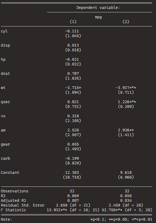

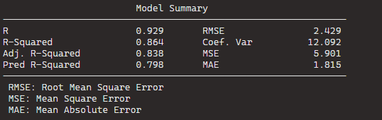
We can see that the stepwise model has only three variables compared to the ten variables in my original model.

And even with far fewer variables, the R2 has decreased by an insignificant amount. In fact the Adjusted R2 increased because we are not being penalised for throwing so many unnecessary variables.

So we can quickly find a model that loses no explanatory power by is far more parsimonious.

Plus in the original model, only one variable is significant but in the stepwise variable all three of the variables are significant.

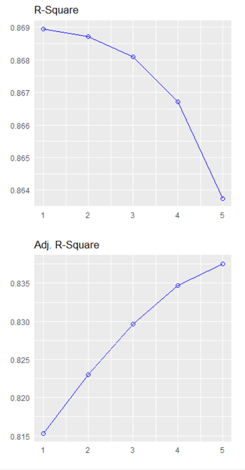
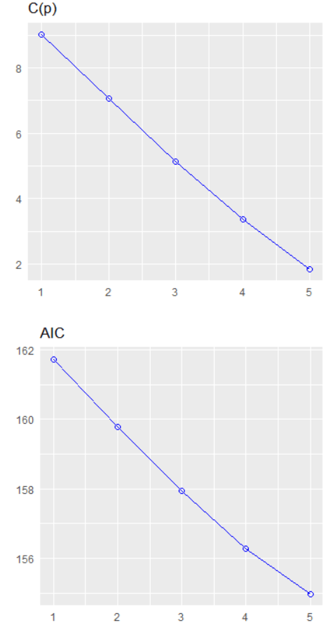
We can plot out the stepwise regression with the oslrr package

car_model %>% 
   ols_step_backward_p() %>% plot()

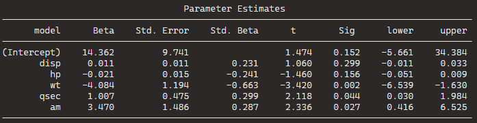
car_model %>% 
   ols_step_backward_p(details = TRUE)

With this, we can iterate over the steps. First, we can look at the first step:

The removal of cyl suggests that, after evaluating its p-value, it was found to be not statistically significant in predicting the response variable.

The model is iteratively refining itself by removing variables that do not provide significant information.

In total, it runs five steps and we arrive at the final step and the final model.

Below, we can look at the Final Model Output: