How to download and animate the Varieties of Democracy (V-DEM) dataset in R

In this blog post, we will download the V-DEM datasets with their vdemdata package. It is still in development, so we will use the install_github() function from the devtools package

devtools::install_github("vdeminstitute/vdemdata")

library(vdemdata)

And really quickly we can download the dataset with one line of code

vdemdata::vdem -> vdem

We can use the find_var function to get information on variables based on keywords.

For example, we can look up variables that are concerned with protest mobilization.

vdemdata::find_var("mobilization") -> mob
 mob %>% names
 [1] "question_id"              "question_number"          "metasection"             
 [4] "name"                     "vartype"                  "cb_section"              
 [7] "tag"                      "projectmanager"           "question"                
[10] "clarification"            "responses"                "ordering"                
[13] "scale"                    "answertype"               "sources"                 
[16] "notes"                    "datarelease"              "citation"                
[19] "coverage"                 "subsetof"                 "crosscoder_aggregation"  
[22] "aggregation"              "ccp_tag"                  "clean_tag"               
[25] "survey_id"                "vignettes_used"           "old_tag"                 
[28] "compiler"                 "clarification_historical" "codebook_id"             
[31] "conthistmerge"            "histmerged"               "years"                   
[34] "hist_outside_coding"      "additional_versions"      "cleaning"                
[37] "date_specific"            "available_versions"       "cont_outside_coding"     
[40] "overlap_use_hist"         "is_party"                 "cb_section_type"         
[43] "defaultdate"              "convergence"              "cy_aggregation"          
[46] "no_update" 

Or download the entire codebook:

vdemdata::codebook -> vdem_codebook

And we can look at information for a specific variable

vdemdata::var_info("e_regionpol_6C") -> region_info 
region_info$responses
1: Eastern Europe and Central Asia (including Mongolia and German Democratic Republic)
2: Latin America and the Caribbean
3: The Middle East and North Africa (including Israel and Türkiye, excluding Cyprus)
4: Sub-Saharan Africa
5: Western Europe and North America (including Cyprus, Australia and New Zealand, but excluding German Democratic Republic)
6: Asia and Pacific (excluding Australia and New Zealand; see 5)"

For our analysis, we can focus on the years 1900 to 2022.

vdem %<>% 
  filter(year %in% c(1900:2022))

And we will create a ggplot() object that also uses the Five Thirty Eight theme from the ggthemes package.

Click here to read more about the ggthemes options.

Source: https://yutannihilation.github.io/allYourFigureAreBelongToUs/ggthemes/

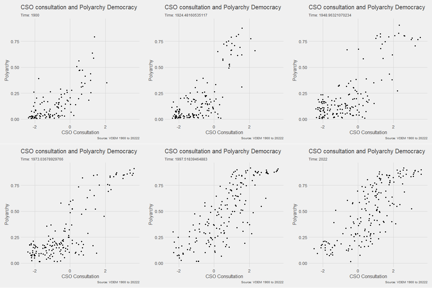
In the V-DEM package, we will look at a scatterplot of CSO consultation (v2cscnsult) and democracy score (v2x_polyarchy).

  • v2cscnsult asks are major civil society organizations (CSOs) routinely consulted by policymakers on policies relevant to their members?
  • v2x_polyarchy examines to what extent is the ideal of electoral democracy in its fullest sense achieved?

First, find below the packages we will need to install and load

install.packages("gganimate")
install.packages("transformr")  # sometimes needed as a dependency

library(gganimate)

And we plot our graph:

my_graph <- ggplot(vdem, aes(x = v2cscnsult, 
                      y = v2x_polyarchy, 
                      group = year)) +
  geom_point()  +
  ggthemes::theme_fivethirtyeight() +
  theme(text = element_text(size = 12),  # Default text size for all text elements
        plot.title = element_text(size = 20, face="bold"),  
        axis.title = element_text(size = 16), 
        axis.text = element_text(size = 14), 
        legend.title = element_text(size = 14),  
        legend.text = element_text(size = 12))  

In the themes argument, we can change the size of the text for the various parts of the ggplot (legends, axes etc.)

To make the ggplot object animated, we use the transition_time(year) function from the gganimate package.

Also we can add a subtitle the displays the year and time frame in the graph.

animated_graph <- my_graph +
  transition_time(year) +
  labs(title = "CSO consultation and Polyarchy Democracy",
       subtitle = "Time: {frame_time}",
       caption = "Source: VDEM 1900 to 2022",
       x = "CSO Consultation",
       y = "Polyarchy")

And we can change how we render the graph with the animate() function.

We choose duration = 15 so that the gif lasts 15 seconds

We set frames per second to 20 fps (the higher the number, the smoother the gif changes, but the longer it takes to load)

And finally we can choose a special renderer that makes the gif more smooth too.

Finally we can save the gif to our computer (so I can upload it here on this blog)

animate(animated_plot, duration = 15, fps = 20, renderer = gifski_renderer()) -> CSO_poly_gif

anim_save("animated_plot.gif", animation = CSO_poly_gif)
We can make a few changes so that it is divided by region and adds colors:

Notice the change to subtitle = "Year: {as.integer(frame_time)}" so it only uses the year, not the year and frame rate.

ggplot(vdem, aes(x = v2cscnsult, 
                      y = v2x_polyarchy, 
                      group = year,
                 size = e_pop, 
                 colour = as.factor(e_regionpol_6C))) +
  geom_point(alpha = 0.7, show.legend = FALSE) +
  ggthemes::theme_fivethirtyeight() +
  theme(text = element_text(size = 12),  
        plot.title = element_text(size = 20, face="bold"), 
        axis.title = element_text(size = 16),  
        axis.text = element_text(size = 14),  
        legend.title = element_text(size = 14),  
        legend.text = element_text(size = 12)) +
  facet_wrap(~e_regionpol_6C) +
  transition_time(year) +
  labs(title = "CSO consultation and Polyarchy Democracy",
       subtitle = "Year: {as.integer(frame_time)}",
       caption = "Source: VDEM 1900 to 2022",
       x = "CSO Consultation",
       y = "Polyarchy")  

Next, we can animate a map

library(sf)
library(rnaturalearth)

First we download a world object with the longitude and latitude data we need.

Click here to read more about the rnaturalearth package

my_map <- ne_countries(scale = "medium", returnclass = "sf")

And we merge the two data.frames together

my_map %<>% 
  mutate(COWcode = countrycode::countrycode(sovereignt, "country.name", "cown"))

vdem_map <- left_join(vdem, my_map, by = c("COWcode"))

Set up some colors for the map

colors <- c("#001427", "#708d81", "#f4d58d", "#bf0603", "#8d0801")

Next we draw the map:

vdem_map %>% 
  filter(year %in% c(1945:2023)) %>% 
  filter(sovereignt != "Antarctica") %>% 
  group_by(country_name, geometry) %>% 
  summarise(avg_polyarchy = mean(v2x_polyarchy, na.rm = TRUE)) %>% 
  ungroup() %>% 
  ggplot() +
  geom_sf(aes(geometry = geometry, fill = avg_polyarchy),  
          position = "identity", color = "#212529", linewidth = 0.2, alpha = 0.85) +
  geom_tile(data = data.frame(value = seq(0, 1, length.out = length(colors))), 
            aes(x = 1, y = value, fill = value), 
            show.legend = FALSE) +
  scale_fill_gradientn(colors = colors, 
                       breaks = scales::pretty_breaks(n = length(colors)),
                       labels = scales::number_format(accuracy = 1)) +
  theme_minimal()

When I made the first attempt to animate the polyarchy democracy data on the map, it was a bit of an affront to the senses:

So attempt number two involved a bit more wrangling!

vdem_map %>% 
  filter(year %in% c(1945:2023)) %>% 
  filter(sovereignt != "Antarctica") %>% 
  ggplot() +
  geom_sf(aes(geometry = geometry, fill = v2x_polyarchy, group = year),  
          position = "identity", color = "#212529", linewidth = 0.2, alpha = 0.85) +
  theme_minimal() +
  scale_fill_gradientn(colors = colors,
                       breaks = scales::pretty_breaks(n = length(colors)),
                       labels = scales::number_format(accuracy = 3)) +
  transition_time(year) + 
  labs(title = "Polyarchy Democracy annual global changes",
       subtitle = "Year: {as.integer(frame_time)}",
       caption = "Source: VDEM 1900 to 2023",
       x = " ",
       y = " ",
       fill = "Democracy Score")  -> my_plot

animate(my_plot, duration = 40, fps = 40,
        renderer = gifski_renderer()) -> map_gif

anim_save("animated_plot_3.gif", animation = map_gif)

Tips and code snippets to improve ggplot graphs and plots in R

Some code snippets to improve graph appearance and readability!

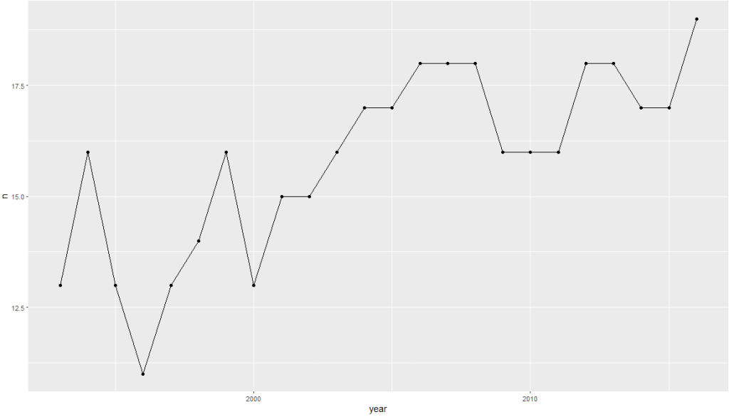
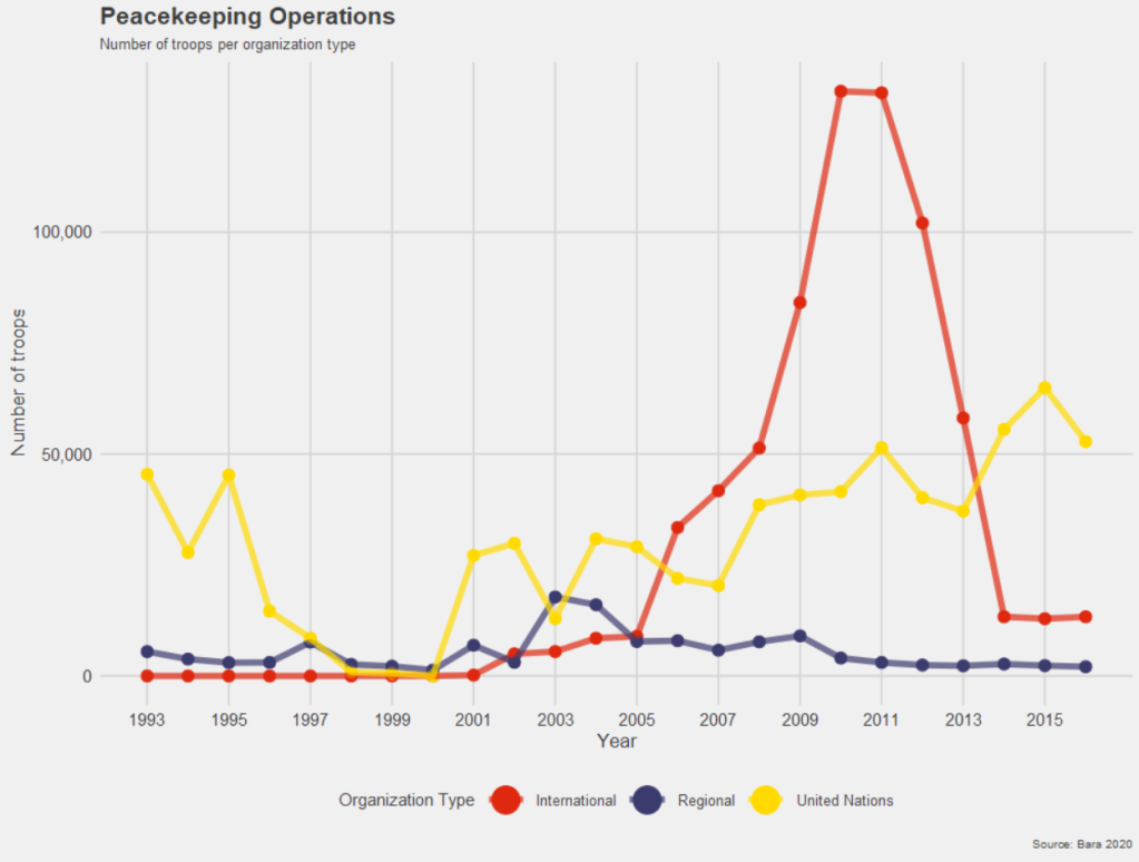
Compare the first basic graph with the second more informative graph.

Happy Birthday Reaction GIF - Find & Share on GIPHY
pko %>% 
  group_by(year) %>% 
  count() -> ya

ya %>% 
  ggplot(aes(x = year,
             y = n)) +
  geom_point() + geom_line()

Dealing with the z and y axes can be a pain.

yo %>% 
  ggplot(aes(x = year, y = n)) + 
  geom_point() + 
  geom_line() +
  scale_x_continuous(breaks = seq(min(yo$year, na.rm = TRUE), 
                                  max(yo$year, na.rm = TRUE), 
                                  by = 1)) + 
  scale_y_continuous(limits = c(0, max(yo$n, na.rm = TRUE)),
                     breaks = function(limits) seq(floor(limits[1]), ceiling(limits[2]), by = 1)
  )

In this code:

The breaks argument of scale_y_continuous() is set using a custom function that takes limits as input (which represents the range of the y-axis determined by ggplot2 based on your data).

seq() generates a sequence from the floor (rounded down) of the minimum limit to the ceiling (rounded up) of the maximum limit, with a step size of 1.

This ensures that the sequence includes only whole integers.

Using floor() for the start of the sequence ensures you start at a whole number not greater than the smallest data point, and ceiling() for the end of the sequence ensures you end at a whole number not less than the largest data point.

This approach allows the y-axis to dynamically adapt to your data’s range while ensuring that only whole integers are used as ticks, suitable for counts or other integer-valued data.

pko %>% 
  pivot_longer(!c(cown, year),
               names_to = "organization",
               values_to = "troops") %>% 
  group_by(year, organization) %>% 
  summarise(sum_troops = sum(troops, na.rm = TRUE)) %>% 
  ungroup() -> yo


pal <- c("totals_intl" = "#DE2910",
         "totals_reg" = "#3C3B6E", 
         "totals_un" = "#FFD900")

yo %>% 
  ggplot(aes(x = year, y = sum_troops,
             group = organization,
             color = organization)) + 
  geom_point(size = 3) +
  geom_line(size = 2, alpha = 0.7)  + 
  scale_y_continuous(labels = scales::label_comma()) + 
  # scale_y_continuous(limits = c(0, max(yo$n, na.rm = TRUE))) +
  scale_x_continuous(breaks = seq(min(yo$year, na.rm = TRUE), 
                                  max(yo$year, na.rm = TRUE), 
                                  by = 2)) +
  ggthemes::theme_fivethirtyeight() +
  scale_color_manual(values =  pal,
                     name = "Organization Type",  
                     labels = c("International",
                                "Regional",
                                "United Nations")) +
  labs(title = "Peacekeeping Operations",
       subtitle = "Number of troops per organization type",
       caption = "Source: Bara 2020",
       x = "Year",
       y = "Number of troops") +
  
  guides(color = guide_legend(override.aes = list(size = 8))) + 
  theme(text = element_text(size = 12),  # Default text size for all text elements
        plot.title = element_text(size = 20, face="bold"),  # Plot title
        axis.title = element_text(size = 16),  # Axis titles (both x and y)
        axis.text = element_text(size = 14),  # Axis text (both x and y)
        legend.title = element_text(size = 14),  # Legend title
        legend.text = element_text(size = 12))  # Legend items

Cairo::CairoWin()    
Happy Season 5 GIF by The Office - Find & Share on GIPHY

Next, we will look at changing colors in our maps.

We have a map and we want to make the colors pop more.

Click here to read about downloading the V-DEM and map data:

   geom_tile(data = data.frame(value = seq(0, 1, length.out = length(colors))), 
             aes(x = 1, y = value, fill = value), 
             show.legend = FALSE) +
   scale_fill_gradientn(colors = colors, 
                        breaks = scales::pretty_breaks(n = length(colors)),
                        labels = scales::number_format(accuracy = 1)) +

Creation of data for geom_tile():

data = data.frame(value = seq(0, 1, length.out = length(colors))) 

This line creates a data.frame with a single column named value. The column contains a sequence of values from 0 to 1. The length.out parameter is set to the length of the colors vector, meaning the sequence will be of the same length as the number of colors you have defined. This ensures that the gradient will have the same number of distinct colors as are in your colors vector.

geom_tile()

geom_tile(aes(x = 1, y = value, fill = value), show.legend = FALSE)

geom_tile() is used here to create a series of rectangles (tiles). Each tile will have its y position set to the corresponding value from the sequence created earlier. The x position is fixed at 1, so all tiles will be in a straight line. The fill aesthetic is mapped to the value, so each tile’s fill color will be determined by its y value. The show.legend = FALSE parameter hides the legend for this layer, which is typically used when you want to create a custom legend.

scale_fill_gradientn()

scale_fill_gradientn(colors = colors, breaks = scales::pretty_breaks(n = length(colors)), labels = scales::number_format(accuracy = 1)) 

scale_fill_gradientn() creates a color scale for the fill aesthetic based on the colors vector that we supplied.

The breaks argument is set with scales::pretty_breaks(n = length(colors)), which calculates ‘pretty’ breaks for the scale, basically nice round numbers within the range of your data, and it is set to create as many breaks as there are colors.

The labels argument is set with scales::number_format(accuracy = 2), which specifies how the labels on the legend should be formatted. The accuracy = 2 parameter means that the labels will be formatted to one decimal place

Random coding tips I always forget: 50+ tips for tidyverse, purrr, stringr, lubridate, janitor and other packages

Packages we will need:

library(rnaturalearth)
library(tidyverse)
library(skimr)
library(lubridate)
library(magrittr)

I use this post to keep code bits all in one place so I can check back here when I inevitably forget them.

Forget Will Smith GIF - Find & Share on GIPHY

For most of the snippets, we can use a map data.frame that we can download from the rnaturalearth package. So the code below downloads a map of the world.

my_map <- ne_countries(scale = "medium", returnclass = "sf")

my_map %>% View

my_map %<>% select(sovereignt,
iso_a2,
pop_est,
gdp_md_est,
economy,
income_grp,
region_un:region_wb)

my_map %<>% select(-geometry) %>% as_tibble()
  1. How to KEEP only one data.frame from the R environment.
all_objects <- ls()
objects_to_remove <- setdiff(all_objects, "my_map")
rm(list = objects_to_remove, envir = .GlobalEnv)

2. Add an ID variable based on row number

my_map %<>% mutate(id = row_number())

3. Replace NAs across all the df with 0 (also using the assignment operator from magrittr pacakge)

my_map %<>% 
  mutate_all(~replace_na(., 0))

4. Plot missing variables in a data.frame

library(DataExplorer)
plot_missing(my_map)

5. Summarise all variables with skimr package

library(skimr)
skim(df)

6. Reverse score a variable

df %>%
mutate(reversed_score_var = max(score_var) + min(score_var) - score_var)

Lots and lots of stringr package stuff (and a bit of regex)

7. To remove footnote brackets – like [4] and [11] - from a string

 df <- df %>%
mutate(column = str_replace_all(column, "\\[[0-9]+\\]", ""))

\\[ : Matches the opening square bracket

[0-9]+ : Matches one or more digits

\\]: Matches the closing square bracket

8. Remove a string pattern from all variables in a data.frame

my_map %<>%
rename_all(~str_remove(., "_map"))

9. How to extract s substring based on a pattern

my_map %<>%
mutate(my_pattern_substring = str_extract(my_string_variable, "my_pattern"))

10. To concatenate (link together) strings

str_c("a", "b", "c") 
[1] "abc"

11. And how to compute the length of strings

str_length("abcdefme")  
[1] 8

12. Extract substrings from a character variable

my_map %<>% 
mutate(income_substring = substr(income_grp,
start = 1, stop = 3))

13. Split a string into pieces

str_split("a,b,c", ","str_split("Merry, Christmas, to, you", ",")  
[[1]]
[1] "Merry"      " Christmas" " to"        " you" 

14. Replace matched patterns in a string

my_map %<>% 
mutate(earning_grp =str_replace(income_grp, "income", "earning"))
1 4. Lower middle earning     60
2 3. Upper middle earning     58
3 2. High earning: nonOECD    46
4 5. Low earning              42
5 1. High earning: OECD       35

15. Detect the presence or absence of a pattern

my_map %<>% 
mutate(asia = str_detect(region_wb, "Asia"))
  asia      n

1 FALSE   127
2 TRUE    114

16. Count the number of occurrences of a pattern

   oecd     n

1 0 160
2 1 81

17. Trim leading and trailing whitespace

str_trim("   abc   ")

Leaving stringr, back to other random code bits

18. Calculates the sum of values across all columns for each row in a data.frame

df %>% rowwise() %>%
mutate(sum = sum(c_across(everything())))

19. Using reduce() function from purrr package to iteratively combine elements in a vector

character_vector <- c("Good", "Will ", "Hunting")

reduce(character_vector, paste0)

20. Finding the maximum value in the disp column

reduce(mtcars$disp, pmax)

Map package code bits

21. Applying a summary function across variables in a data.frame

summary_stats_fun <- function(df, var, grouping_var) {
result <- df %>%
group_by({{ grouping_var }}) %>%
summarise(
count = n(),
sum_var = sum({{ var }}, na.rm = TRUE)
) %>%
arrange(desc(count))
return(result)
}

map_summary_stats <- function(list_of_data, var, grouping_var) {
result <- map(list_of_data, ~ summary_stats_fun(.x, var = var, grouping_var = grouping_var))
return(result)

}

list_of_data <- list(
data.frame(country = c("A", "B", "A", "C", "B", "C"), value = c(10, 15, 20, 5, 8, 12)),
data.frame(country = c("A", "A", "B", "B", "C", "C"), value = c(8, 12, 15, 10, 5, 20))
)

result_summary_stats <- map_summary_stats(list_of_data, var = "value", grouping_var = "country")

22. How to remove rows from a data.frame that match a string pattern

df <- df %>%
filter(!grepl("pattern", column))

23. How to remove non-numeric characters

df <- df %>%
mutate(column = str_replace_all(column, "[^0-9]", ""))

24. Removing parentheses and contents within

df <- df %>%
mutate(column = str_replace_all(column, "\\(.*?\\)", ""))

25. How to split a string into two new variables

df <- df %>%
separate(column, into = c("new_col_1", "new_col_2"), sep = ",
")

26. Extracting alphabetic characters

df <- df %>%
mutate(alpha_chars = str_extract_all(column, "[A-Za-z]"))

27. Remove scientific notation

old_scipen <- options("scipen") # Save the current scipen value
options(scipen = 999) # Disable scientific notation
options(old_scipen) # Reset

Some functions from the forcats package for factor variables

28. Count the occurrences of each level in a factor

fct_count(factor_variable)

29. Order levels by their frequency.

fct_infreq(factor_variable)

30. Lump levels into a specified number of top or bottom levels.

fct_lump(factor_variable, n = 5)

31. Collapse factor levels into broader categories.

fct_collapse(factor_variable, new_levels = c("Category1", "Category2"))

32. Relabel factor levels

fct_relabel(factor_variable, new_labels = c("Label1", "Label2"))

33. Reverse the order of factor levels.

fct_rev(factor_variable)

34. Make NAs explicit by adding a level for missing values.

fct_explicit_na(factor_variable)

35. Group infrequent levels into “Other” category.

fct_other(factor_variable, keep = 5)

36. Create a cross-tabulation of two factors.

fct_cross(factor1, factor2)

37. Recode factor levels.

fct_recode(factor_variable, new_levels = c("NewLevel1" = "OldLevel1", "NewLevel2" = "OldLevel2"))

38. Count the occurrences of each level in a factor.

fct_count(factor_variable)

And next we will look at lubridate functions I always need to look up. Dates are a pain.

39. Parse date character in the “Year-Month-Day” format.

ymd("2023-12-16")

40. Get the current date and time.

now()

41. Get the current date only

today()

42. How to extract a year from a date class.

year(ymd("2023-12-16"))

43. And to extract the hour from the time now

hour(now())

44. How to extrac the day of the week from a data class

wday(ymd("2023-12-16"))

45. Rounding up or rounding down to the nearest time unit

floor_date(now(), "months")

ceiling_date(now(), "hours")

46. Create an interval object.

my_interval <- interval(start = ymd("2023-01-01"), end = ymd("2023-12-31"))

47. Get the timezone of date and time now

timezone(now())

And last the janitor package for cleaning variables

48. Clean names with lowercase letters and _underscores_

library(janitor)
cleaned_data <- clean_names(original_data)

49. Clean and remove away empty rows and columns from a data.frame

cleaned_data <- remove_empty(original_data)

50. How to remove columns with constant values

cleaned_data <- remove_constant(original_data)

51. How to find duplicate rows in a data.frame

duplicate_rows <- get_dupes(original_data, columns = c("col1", "col2"))

52. How to add percentage sign (%) to a contingency table

table_with_percentages <- tabyl(original_data, col1, col2) %>%
adorn_percentages("row")

53. Add row or column counts to a contingency table

table_with_counts <- tabyl(original_data, col1, col2) %>%
adorn_ns()

54: Changing Data Types

df %>%
mutate(across(starts_with("num"), as.character))

55. Scaling Numeric Variables

df %>%
mutate(across(where(is.numeric), scale))

56. Applying a Custom Function

df %>%
mutate(across(contains("price"), ~ .x * 1.1))

57. Filter based on a condition

df %>%
filter(across(ends_with("score"), ~ .x > 80))

58. Inpute a missing variable

df %>%
mutate(across(starts_with("var"), ~ifelse(is.na(.x), mean(.x, na.rm = TRUE), .x)))

59. Selecting Columns with Specific Data Types:

df %>%
select(across(where(is.character)))

60. Rename columns with paste()

df %>%
rename(across(contains("old"), ~ paste0("new_", .x)))

61. How to calculate row sums

df %>%
mutate(total = rowSums(across(starts_with("quantity"))))

62. Group-wise scaling

df %>%
group_by(category) %>%
mutate(across(starts_with("value"), scale))

63. How to conditionally mutate

  df %>% mutate(across(starts_with("sales"), ~ ifelse(.x > 100, "High", "Low")))

64. Output tidy regression model without scientific notatio

plm(lead(dep_var, 2) ~ ind_var, index = c("country", "year"), 
data = df) %>%
broom::tidy() %>%
arrange(desc(estimate)) %>%
mutate(across(c(estimate, std.error, statistic, p.value), ~sprintf("%.10f", .)))
print(n = 100)

65. How to choose the reference factor for a regression

df %<>%
mutate(factor_var = relevel(as.factor(factor_var), ref = "ref_level"))

66. Remove variables that end with a character string.

vdem %<>%
select(-ends_with("_sd"),
-ends_with("_codelow"),
-ends_with("_codehigh"),
-ends_with("_3C"),
-ends_with("_4C"),
-ends_with("_5C"))

Can you add more code snippets in the commets???

Schitts Creek Yes GIF by CBC - Find & Share on GIPHY

Include country labels to a regression plot with ggplot2 package in R

Sometimes the best way to examine the relationship between our variables of interest is to plot it out and give it a good looking over. For me, it’s most helpful to see where different countries are in relation to each other and to see any interesting outliers.

For this, I can use the geom_text() function from the ggplot2 package.

I will look at the relationship between economic globalization and social globalization in OECD countries in the year 2000.

The KOF Globalisation Index, introduced by Dreher (2006) measures globalization along the economicsocial and political dimension for most countries in the world

First, as always, we install and load the necessary package. This time, it is the ggplot2 package

install.packages("ggplot2")
library(ggplot2)

Next add the following code:

fin <- ggplot(oecd2000, aes(economic_globalization, social_globalization)) 
        + ggtitle("Relationship between Globalization Index Scores among OECD countries in 2000")
        + scale_x_continuous("Economic Globalization Index")
        + scale_y_continuous("Social Globalization Index") 
        + geom_smooth(method = "lm") 
        + geom_point(aes(colour = polity_score), size = 2) + labs(color = "Polity Score")
        + geom_text(hjust = 0, nudge_x = 0.5, size = 4, aes(label = country)) 

fin 

In the aes() function, we enter the two variables we want to plot.

Then I use the next three lines to add titles to axes and graph

I use the geom_smooth() function with the “lm” method to add a best fitting regression line through the points on the plot. Click here to learn more about adding a regression line to a plot.

I add a legend to examine where countries with different democracy scores (taken from the Polity Index) are located on the globalization plane. Click here to learn about adding legends.

The last line is the geom_text() function that I use to specify that I want to label each observation (i.e. each OECD country) with its name, rather than the default dataset number.

Some geom_text() commands to use:

  • nudge_x (or nudge_y) slightly “nudge” the labels from their corresponding points to help minimise messy overlapping.
  • hjust and vjust move the text label “left”, “center”, “right”, “bottom”, “middle” or “top” of the point.

Yes, yes! There is a package that uses the color palettes of Wes Anderson movies to make graphs look just beautiful. Click here to use different Wes Anderson aesthetic themed graphs!

zissou_colors <- wes_palette("Zissou1", 100, type = "continuous")

fin + scale_color_gradientn(colours = zissou_colors)

Which outputs:

Interestingly, it seems that at the very bottom left hand corner of the plot (which shows the countries that are both low in economic globalization and low in social globalization), we have two OECD countries that score high on democracy – Japan and South Korea- right next to two countries that score the lowest in the OECD on democracy, Turkey and Mexico.

So it could be interesting to further examine why these countries from opposite ends of the democracy spectrum have similar pattern of low globalization. It puts a spanner in the proverbial works with my working theory that countries higher in democracy are more likely to be more globalized! What is special about these two high democracy countries that gives them such low scores on globalization.

Create facetted scatterplots with the ggplot2 package in R

If I want to graphically display the relationship between two variables, the ggplot2 package is a very handy way to produce graphs.

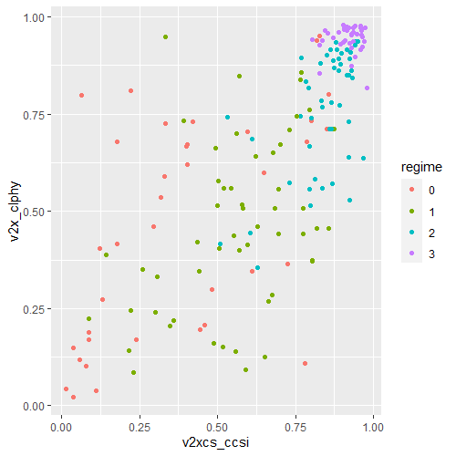
For example, I can use the ggplot2 package to graphically examine the relationship between civil society strength and freedom of citizens from torture. Also I can see whether this relationship is the same across regime types.

I choose one year from my dataframe to examine.

data2000 <- myPanel[which(myPanel$year == "2000"),]

Next, I install the ggplot2 package

install.packages("ggplot2")
library(ggplot2)

The grammar of ggplot2 includes:

  • aes() indicates how variables are mapped to visual properties or aesthetics. The first variable goes on the x-axis and the second variable goes on the y-axis.
  • geom_point() creates a scatterplot style graph. Alternatives to this are geom_line(), which creates a line plot and geom_histogram() which creates a histogram plot.

ggplot(data2000, aes(v2xcs_ccsi, v2cltort)) + geom_point() +
xlab("Civil society robustness") +
ylab("Freedom from torture")

Next we can add information on regime types, a categorical variable with four levels.

0 = closed autocracy

1 = electoral autocracy

2 = electoral democracy

3 = liberal democracy

In the aes() function, add colour = regime to differentiate the four categories on the graph

ggplot(data2000, aes(v2xcs_ccsi, v2x_clphy, colour = regime)) +
geom_point()

Alternatively we can use the facet_wrap( ~ regime) function to create four separate scatterplots and examine the relationship separately.

ggplot(data2000, aes(v2xcs_ccsi, v2x_clphy, colour = regime)) +
geom_point() +
facet_wrap(~regime) +
xlab("Civil society robustness") +
ylab("Freedom from torture")

Lastly, we can add a linear model line (method = "lm") with a grey standard error bar (se = TRUE) in the geom_smooth() function.

ggplot(data2000, aes(v2xcs_ccsi, v2x_clphy, colour = regime)) +
geom_point() +
facet_wrap(~regime) +
geom_smooth(method = "lm", se = TRUE) +
xlab("Civil society robustness") +
ylab("Freedom from torture")

In these graphs, we can see that as civil society robustness score increases, the likelihood of a life free from torture increases! Pretty intuitive result and we could argue that there is a third variable – namely strong democratic institutions – that drives this positive relationship.

The graphs break down this relationship across four different regime types, ranging from the most autocratic in the top left hand side to the most democratic in the bottom right. There is more variety in this relationship with closed autocracies (i.e. the red points), with some points deviating far from the line.

The purple graph – liberal democracies – shows a tiny amount of variance. In liberal democracies, it appears that all countries score highly in both civil society robustness and freedom from torture!

Turn wide to long format with reshape2 package in R

A simple feature to turn wide format into long format in R.

I have a dataset with the annual per capita military budget for 171 countries.

The problem is that it is in completely wrong format to use for panel data (i.e. cross-sectional time-series analysis).

So here is simple way I found to fix this problem and turn this:

WIDE FORMAT : a separate column for each year

into this:

LONG FORMAT : one single “year” column and one single “value” column

It’s like magic.

First install and load the reshape2 package

install.packages("reshape2")
library(reshape2)

I name my new long form dataframe; in this case, the imaginatively named mil_long.

I use the melt() function and first type in the name of the original I want to change; in this case it is mil_wide

id.vars tells R the unique ID for each new variable. Since I am looking at military budgets for each country, I’ll use Country variable as my ID.

variable.name for me is the year variable which, in wide format, is the name of every column. For me, I want to compress all the year columns into this new variable.

value.name is the new variable I make to hold the value that in my dataset is the per capita military budget amount per country per year. I name this new variable … you guessed it, value.

mil_long <- melt(mil_wide, id.vars= "Country", variable.name = "year", value.name = "value"))

So simple, it’s hard to believe.

Looking at my new mil_long dataset, my new long format dataframe has only three columns = “Country”, “year” and “value” and 5,504 rows for each country-year observation across the 32 years.

Now, my dataframe is ready to be transformed into a panel data frame!

reshape2 has two main functions which I think have quite memorable names:  melt and cast.

melt is for wide-format dataframes that you want to “melt” into long-format.

cast for dataframes in long-format data which you figuratively “cast” into a wide-format dataframe.

As a poli-sci person, I have so far only turned my dataframe in long form, for eventual panel data analysis with "plm" package.

Click here to see how to transform dataframes into panel dataframes with the plm package.

Click here to read the full reshape2 package documentation on CRAN