Building a dataset for political science analysis in R, PART 1

When you want to create a dataset for large-n political science analysis from scratch, it can get muddled fast. Some tips I have found helpful to create clean data ready for panel data analysis.

Click here for PART 2 to create dyad-year and state-year variables with conflict, geographic features and alliance data from Correlates of War and Uppsala datasets.

Packages we will need

library(tidyverse)  # of course!
library(states)
library(WDI)
library(countrycode)
library(rnaturalearth)
library(VIM)

The states package by Andreas Beger can provide the skeleton for our panel dataset.

It create a cross-sectional, time-series dataset of independent sovereign countries that stretch back to 1816.

The package includes both the Gleditsch & Ward (G&W) and Correlates of War (COW) lists of independent states.

Click here for a discussion of the difference by Stephen Miller.

With the state_panel function from the states package, we create a data.frame from a start date to an end date, using the following syntax.

state_panel(start, end, by = NULL, partial = "any", useGW = TRUE)

The partial argument indicates how we want to deal with states that is independent for only part of the year. We can indicate “any”, “exact”, “first” or “last”.

For this example, I want to create a dataset starting in 1990 and ending in 2020. I put useGW = FALSE because I want to use the COW list of states.

df <- state_panel(1990, 2020, by = "year", partial = "last", useGW = FALSE)
View(df)

And this is the resulting dataset

So we have our basic data.frame. We can see how many states there have been over the years.

df %>% 
  group_by(year) %>% 
  count() %>%  
  arrange(n)

# A tibble: 31 x 2
# Groups:   year [31]
    year     n
   <int> <int>
 1  1990   161
 2  1991   177
 3  1992   181
 4  1993   186
 5  1994   187
 6  1995   187
 7  1996   187
 8  1997   187
 9  1998   187
10  1999   190
11  2000   191
12  2001   191
13  2002   192
14  2003   192
15  2004   192
16  2005   192
17  2006   193
18  2007   193
19  2008   194
20  2009   194
# ... with 11 more rows

We can see that the early 1990s saw the creation of many states after the end of the Soviet Union. Since 2011, the dataset levels out at 195 (after the creation of South Sudan)

Next, we can add the country name with the countrycode() function from the countrycode package. We feed in the cowcode variable and add the full country names. Click here to read more about the function in more detail and see other options to add country ISO code, for example.

df$country <- countrycode(df$cowcode, "cown", "country.name")

With our dataset with all states, we can add variables for our analysis

We can use the WDI package to download any World Bank indicator.

Click here for more information about this super easy package.

I’ll first add some basic variables, such as population, GDP per capita and infant mortality. We can do this with the WDI() function. The indicator code for population is SP.POP.TOTL so we add that to the indicator argument. (If we wanted only a few countries, we can add a vector of ISO2 code strings to the country argument).

POP <- WDI(country = "all",
           indicator = 'SP.POP.TOTL',
           start = 1990, 
           end = 2020)

The default variable name for population is the long string, so I’ll quickly change that

POP$population <- POP$SP.POP.TOTL 
POP$SP.POP.TOTL <- NULL

I’ll do the same for GDP and infant mortality

GDP <- WDI(country = "all",
       indicator = 'NY.GDP.MKTP.KD',
       start = 1990, 
       end = 2020)

GDP$gdp <- GD$PNY.GDP.MKTP.KD
GDP$NY.GDP.MKTP.KD <- NULL

INF_MORT <- WDI(country = "all",
       indicator = 'SP.DYN.IMRT.IN',
       start = 1990, 
       end = 2020)

INF_MORT$infant_mortality <- INF_MORT$SP.DYN.IMRT.IN
INF_MORT$SP.DYN.IMRT.IN <- NULL

Next, I’ll bind all the variables them together with cbind()

wb_controls <- cbind(POP, GDP, INF_MORT)

This cbind will copy the country and year variables three times so we can delete any replicated variables:

wb_controls <- wb_controls[, !duplicated(colnames(wb_controls), fromLast = TRUE)]

When we download World Bank data, it comes with aggregated data for regions and economic groups. If we only want in our dataset the variables for countries, we have to delete the extra rows that we don’t want. We have two options for this.

The first option is to add the cow codes and then filter out all the rows that do not have a cow code (i.e. all non-countries)

wb_controls$cow_code <- countrycode(wb_controls$country, "country.name", 'cown')

Then we re-organise the variables a bit more nicely in the dataset with select() and keep only the countries with filter() and the !is.na argument that will remove any row with NA values in the cow_code column.

df_v2 <- wb_controls %>%
  select(country, iso2c, cow_code, year, everything()) %>%
  filter(!is.na(cow_code))

Alternatively, we can merge the World Bank variables with our states df and it can filter out any row that is not a sovereign, independent state.

In the merge() function, we use by to indicate the columns by which we want to merge the datasets. The all argument indicates which dataset we want to keep and NOT delete rows that do not match. If we typed all = TRUE, it would not delete any rows that do not match.

wb_controls %<>%
  select(cow_code, year, everything()) 

df_v3 <- merge(df, wb_controls, by.x = c("cowcode", "year"), by.y = c("cow_code", "year"), all.x = TRUE)

You can see that df_v2 has 85 more rows that df_v3. So it is up to you which way you want to use, and which countries you want to include each year. The df_v3 contains states that are more likely to be recognised as sovereign. df_v2 contains more territories.

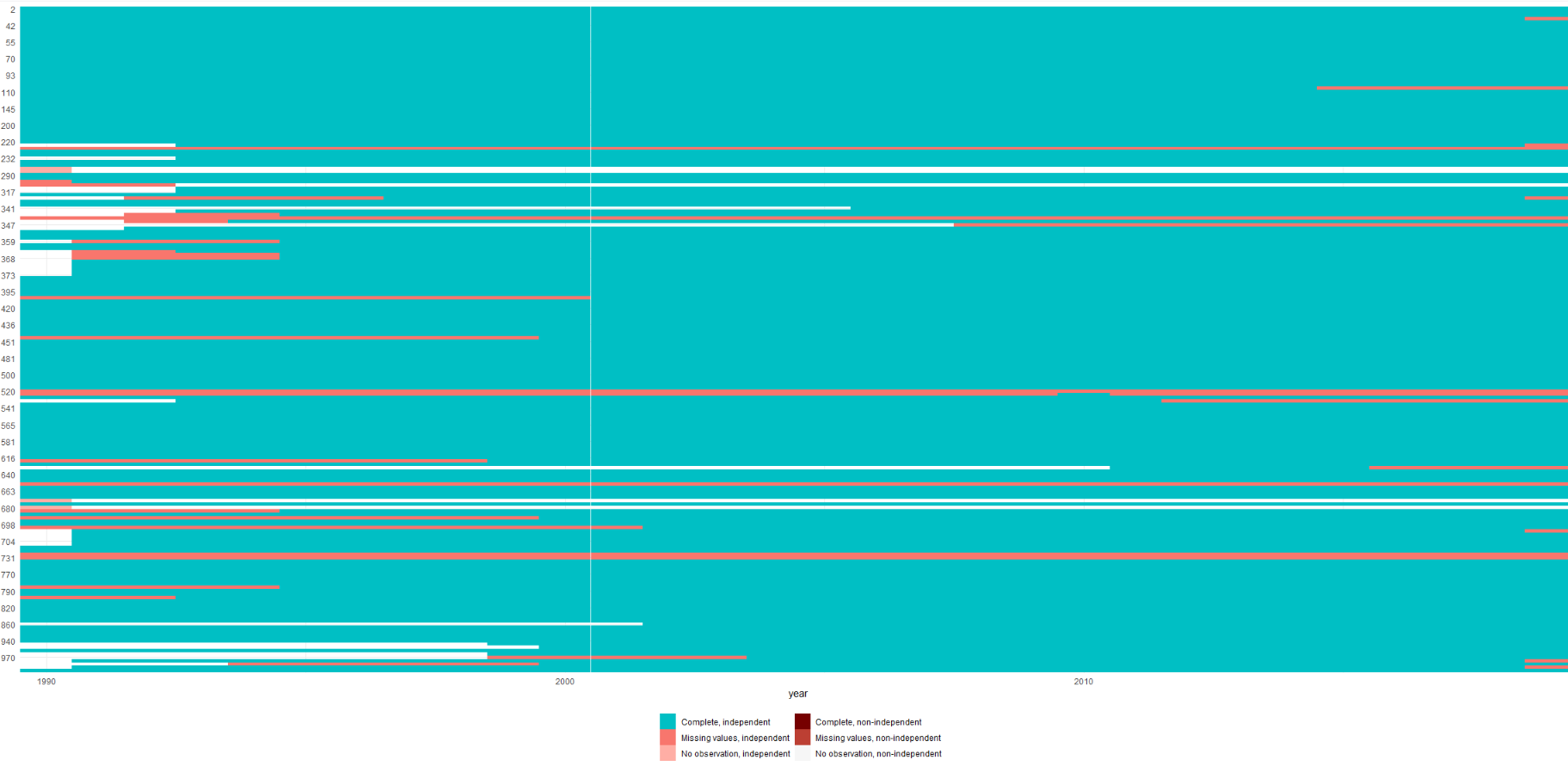
Let’s look at the prevalence of NA values across our dataset.

We can use the plot_missing() function from the states package.

plot_missing(df_v3, ccode = "cowcode")

It is good to see a lot of green!

Let’s add some constant variables, such as geographical information. The rnaturalearth package is great for plotting maps. Click here to see how to plot maps with the package.

For this dataset, we just want the various geography group variables to add to our dataset:

map <- ne_countries(scale = "medium", returnclass = "sf")

We want to take some of the interesting variables from this map object:

map %>% 
  select(admin, economy, income_grp, continent, region_un, subregion, region_wb) -> regions_sf

This regions_sf is not in a data.frame object, it is a simple features dataset. So we delete the variables that make it an sf object and explicitly coerce it to data.frame

regions_sf$geometry<- NULL
regions_df <- as.data.frame(regions_sf)

Finally, we add our COW codes like we did above:

regions_df$cow_code <- countrycode(regions_df$admin, "country.name", "cown")

Warning message:
In countrycode(regions_df$admin, "country.name", "cown") :

Some values were not matched unambiguously: Antarctica, Kashmir, Republic of Serbia, Somaliland, Western Sahara

Sometimes we cannot avoid hand-coding some of our variables. In this case, we don’t want to drop Serbia because the countrycode function couldn’t add the right code.

So we can check what its COW code is and add it to the dataset directly with the mutate function and an ifelse condition:

regions_df %<>% 
  dplyr::mutate(cow_code = ifelse(admin == "Republic of Serbia", 345, cow_code))

If we look at the countries, we can spot a problem. For Cyprus, it was counted twice – due to the control by both Turkish and Greek authorities. We can delete one of the versions because all the other World Bank variables look at Cyprus as one entity so they will be the same across both variables.

regions_df <- regions_df %>% slice(-c(38))

Next we merge the new geography variables to our dataset. Note that we only merge by one variable – the COW code – and indicate that we want to merge for every row in the x dataset (i.e. the first dataset in the function). So it will apply to each year row for each country!

df_v4 <- merge(df_v3, regions_df, by.x = "cowcode", by.y = "cow_code", all.x = TRUE)

So far so good! We have some interesting variables all without having to open a single CSV or DTA file!

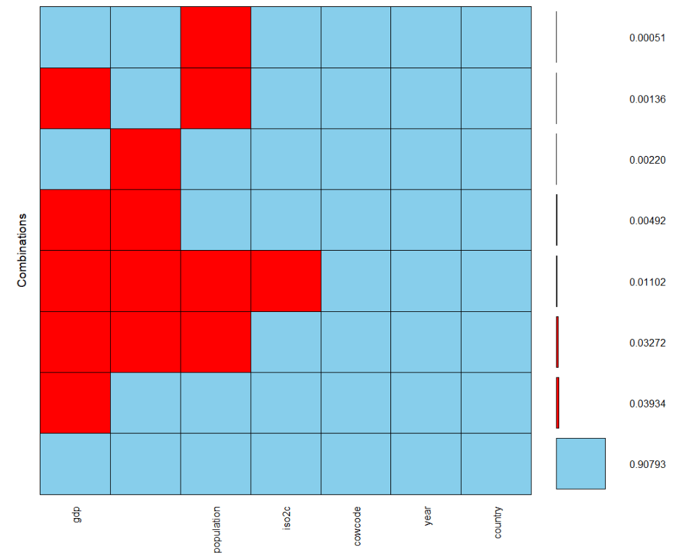
Let’s look at the NA values in the data.frame

nhanes_miss = VIM::aggr(df_v3,
                   labels = names(df_v3), 
                   sortVars = TRUE,
                   numbers = TRUE)

We with the aggr() function from the VIM package to look at the prevalence of NA values. It’s always good to keep an eye on this and catch badly merged or badly specified datasets!