Packages we will need:
library(olsrr)
library(countrycode)
library(WDI)
library(stargazer)
library(peacesciencer)
library(plm)
One core assumption of linear regression analysis is that the residuals of the regression are normally distributed.
When the normality assumption is violated, interpretation and inferences may not be reliable. In worst case, the interpretations are not at all valid.
So it is important we check this assumption is not violated.
As well residuals being normal distributed, we must also check that the residuals have the same variance (i.e. homoskedasticity).
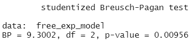
Click here to find out how to check for homoskedasticity.
Then, if there is a problem with the variance, click here to find out how to fix heteroskedasticity (which means the residuals have a non-random pattern in their variance) with the sandwich package in R.
There are three ways to check that the error in our linear regression has a normal distribution:
- plots or graphs such histograms, boxplots or Q-Q-plots, to get a visual approximation
- examining skewness and kurtosis indices
- formal normality tests, to check for a p-value
In this blog, we will see what factors affect military spending by a government.
We will take some variables from the World Bank via the WDI package.
Click here to read more about downloading World Bank Data with the WDI package.
mil_spend_gdp = WDI(indicator = "MS.MIL.XPND.ZS")
gdp_percap = WDI(indicator = "NY.GDP.PCAP.KD")

mil_spend_gdp %>%
  inner_join(gdp_percap) %>%
  select(country, year,
         mil_spend_gdp = MS.MIL.XPND.ZS,
         gdp_percap = NY.GDP.PCAP.KD) %>%
  mutate(cown = countrycode(country, "country.name", "cown")) %>%
  filter(!is.na(cown)) -> wdi_data
And also download some variables via the peacesciencer package.
Click here to read more about the peacesciencer package in the blog posts about building datasets
peacesciencer::create_stateyears(system = "gw") %>%
  add_ucdp_acd() %>%
  add_democracy() %>%
  mutate(cown = countrycode(statename, "country.name", "cown")) -> peace_data
We can code a new binary variable that indicates if there was a UCDP conflict in the previous 10 years or not.
We could imagine a country that experienced war is more likely to keep investing in their military (as a larger percentage of their GDP) than countries that have only experienced relative peace in their recent past.
peace_data %<>%
  select(statename, cown, year, ucdpongoing, maxintensity, conflict_ids, v2x_polyarchy, polity2) %>%
  mutate(ucdpongoing_no_na = ifelse(is.na(ucdpongoing), 0, ucdpongoing)) %>%
  group_by(statename) %>%
  arrange(year) %>%
  mutate(war_past_10_years = ifelse(ucdpongoing == 1 & lag(ucdpongoing, order_by = year, default = 0, n = 10) == 1, 1, 0)) %>%
  mutate(war_past_10_years_no_na = ifelse(ucdpongoing_no_na == 1 & lag(ucdpongoing_no_na, order_by = year, default = 0, n = 10) == 1, 1, 0))
We merge the data by the Correlates of War codes.
Click here to read more about using COW codes with the countrycode package.
wdi_data %>%
  inner_join(peace_data, by = c("cown", "year")) -> wdi_peace
With these data, we can build our linear regression model.
Our dependent variable is military spending as a percentage of GDP (logged)
Our independent varibles are:
- GDP per capita (logged) from the World Bank
- Demoracy (as measured by the V-DEM polyarchy score)
- Binary variable that is 1 if a country had a UCDP conflict in the previous 10 years and 0 if none.
We will also add an interaction term with the GDP and democracy variable.
Given we have cross-sectional longitudinal data, the best option would be panel data analysis with the plm package
plm(log(mil_spend_gdp) ~ log(gdp_percap)*v2x_polyarchy + as.factor(war_past_10_years_no_na), data = wdi_peace,
  index = c("cown", "year"), model = "within") %>%
stargazer(., type = "text")| Dependent variable: | |
| Military spending (GDP %) (ln) | |
| GDP pc (ln) | -0.288*** |
| (0.029) | |
| Democracy | 1.004*** |
| (0.353) | |
| War 10 year dummy | 0.146*** |
| (0.021) | |
| GDP pc (ln) x Democracy | -0.199*** |
| (0.046) | |
| Observations | 3,686 |
| R2 | 0.135 |
| Adjusted R2 | 0.097 |
| F Statistic | 137.989*** (df = 4; 3530) |
| Note: | *p<0.1; **p<0.05; ***p<0.01 |
However, the olsrr package cannot handle plm.
In future blog posts, we will lok more closely at plm() panel regressions and the diagnostic tests we have to run with these types of models.
So we will just look at one year, 2010.
lm(log(mil_spend_gdp) ~ log(gdp_percap)*v2x_polyarchy + as.factor(war_past_10_years_no_na), data = subset(wdi_peace, year == 2010)) -> war_model| Dependent variable: | |
| Military spending (GDP %) (ln) | |
| GDP pc (ln) | 0.261** |
| (0.101) | |
| Democracy | 1.450 |
| (1.565) | |
| War 10 year dummy | 0.592*** |
| (0.159) | |
| GDP pc (ln) x Democracy | -0.343** |
| (0.168) | |
| Constant | 0.183 |
| (0.885) | |
| Observations | 136 |
| R2 | 0.381 |
| Adjusted R2 | 0.362 |
| Residual Std. Error | 0.615 (df = 131) |
| F Statistic | 20.137*** (df = 4; 131) |
| Note: | *p<0.1; **p<0.05; ***p<0.01 |
So now we have our OLS model, we can run a heap of linear model diagnostic functions with the olsrr package.
Built by Aravind Hebbali, the description of the package mentions that olsrr has tools designed to make it easier for users, particularly beginner/intermediate R users to build ordinary least squares regression models. Thank you Aravind!
It includes regression output, heteroskedasticity tests, collinearity diagnostics, residual diagnostics, measures of influence, model fit assessment and variable selection procedures. Look through the CRAN PDF below or look at rsquaredacademy website to get a comprehensive overview of the package
We will now check if the residuals in our model (the difference between what our model predicted and what the values actually are) are normally distributed
ols_test_normality(war_model)| Test | Statistic | p-value |
|---|---|---|
| Shapiro-Wilk | 0.9817 | 0.0653 |
| Kolmogorov-Smirnov | 0.0524 | 0.8494 |
| Cramer-von Mises | 14.1123 | 0.0000 |
| Anderson-Darling | 0.469 | 0.2447 |
Let’s look at each test result in turn
Shapiro-Wilk:
The test statistic is 0.9817, and the p-value is 0.0653.
The null hypothesis is that the residuals are normally distributed.
In this case, the p-value is greater than the predefined significance level (typically 0.05), so you cannot reject the null hypothesis.
This suggests that the residuals may follow a normal distribution.
Woo!
Kolmogorov-Smirnov:
The test statistic is 0.0524, and the p-value is 0.8494.
Similar to the Shapiro-Wilk test, the p-value is greater than 0.05, so you cannot reject the null hypothesis of normality.
This suggests that the residuals may follow a normal distribution.
Yay.
Cramer-von Mises:
This test statistic is 14.1123, and the p-value is 0.0000.
The null hypothesis is that the residuals are normally distributed. The very low p-value indicates that you can reject the null hypothesis, suggesting that the residuals are not from a normal distribution.
Oh no.
Anderson-Darling: This is another test of normality. The test statistic is 0.469, and the p-value is 0.2447. Similar to the Shapiro-Wilk and Kolmogorov-Smirnov tests, the p-value is greater than 0.05, so you cannot reject the null hypothesis of normality.
Phew.
Which of the normality tests is the best?
And what is up with Cramer-von Mises?
A paper by Razali and Wah (2011) tested all these formal normality tests with 10,000 Monte Carlo simulation of sample data generated from alternative distributions that follow symmetric and asymmetric distributions.
Their results showed that the Shapiro-Wilk test is the most powerful normality test, followed by Anderson-Darling test, and Kolmogorov-Smirnov test. Their study did not look at the Cramer-Von Mises test.
The results of Razali and Wah’s study echo the previous findings of Mendes and Pala (2003) and Keskin (2006) in support of Shapiro-Wilk test as the most powerful normality test.
According Ahad and colleagues (2011: 641), they find that
“the performances of the normality tests, namely, the Kolmogorov-Smirnov test, Anderson-Darling test, Cramervon Mises test, and Shapiro-Wilk test, were evaluated under various spectrums of non-normal distributions and different sample sizes. The results showed that the ShapiroWilk test is the most sensitive normality test because this test rejects the null hypothesis of normality at the smallest sample sizes compared to the other tests, at all levels of skewness and kurtosis. Thus, when the four normality tests are available in a statistical package, we would recommend practitioners to use the Shapiro-Wilk normality to test the normality of data”
Ahad et al (2001: 641)
We can plot out the residuals distribution in a histogram with olsrr
olsrr::ols_plot_resid_hist(war_model)
Visually, we can confirm that the residuals have a lovely bell curve and are broadly normally distributed! With a few outliers at -2.
Nest we can check the residuals with a QQ plot.
A QQ plot is used to compare residuals to the normal distribution in linear regression. We can use a normal QQ plot to visually check if our residuals follow a theoretical normal distribution.
In addition to being good at identifying outliers and heavy tails, QQ plots can reveal characteristics such as skewness and bimodality, and can be effective even
for small samples (Marden, 2004).
olsrr::ols_plot_resid_qq(war_model)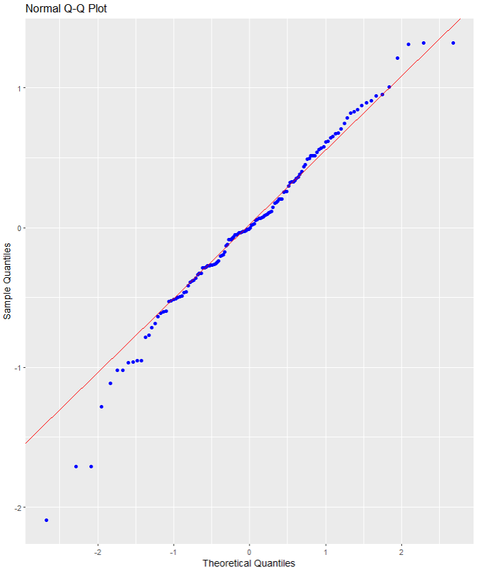
Again we can see some outliers at -2
Next we can look at a scatter plot of residuals on the y axis and fitted values on the x axis to detect non-linearity, unequal error variances, and outliers.
Each point in the plot is a residual value (i.e. the difference between what the model predicted and what the value actually
When interpreting this plot, there are a few things we want to look out for.
- The points does not deviate too far from 0. This indicates the variance is homogeneous (i.e. homescediasticity, one of my favourite words)
- The points are random (i.e. show no distinct pattern) around the horizontal red line at 0
ols_plot_resid_fit(war_model)

- There are some residual values at the -2, so they might be outliers. We we look at an outlier diagnostic plot in a bit.
- There are no discernible pattern in the scatterplot, so there does not seem to be any heteroscedasticity in the variance.
We can run an ols_plot_resid_lev() to graph for detecting outliers and/or observations with high leverage.
ols_plot_resid_lev(war_model)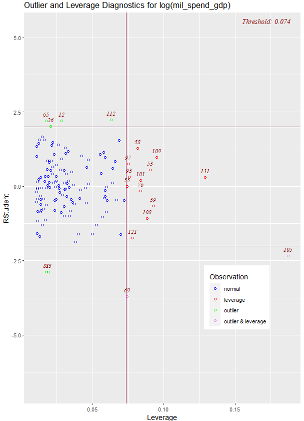
There are a few outliers with leverage that we need to look more closely and examine how they prove / challenge our given theory / hypotheses.
FINALLLY. for a more complete diagnostics check, we can insert the model into the ols_coll_diag() function to calculate the Variance Inflation Factor (VIF) and Eigenvalues of the variables in the model.
VIF scores highlight if there is multicollinearity between the independent variables. If they are too highly correlated, our model is in trouble.
- If the value of VIF is 1< VIF < 5, it specifies that the variables are moderately correlated to each other.
- The challenging value of VIF is between 5 to 10 as it specifies the highly correlated variables.
- If VIF ≥ 5 to 10, there will be multicollinearity among the predictors in the regression model.
- VIF > 10 indicate the regression coefficients are feebly estimated with the presence of multicollinearity
Read more about the issues with multicollinearity in Shrestha (2020)
ols_coll_diag(war_model) | Variables | Tolerance | VIF |
|---|---|---|
| GDP per capita (ln) | 0.13 | 7.6 |
| Democracy | 0.02 | 56.2 |
| War 10 years | 0.91 | 1.1 |
| GDP pc (ln) X Democracy | 0.01 | 79.9 |
Next we look at the Eigenvalues
| Eigenvalue | Condition Index | intercept | GDP pc (ln) | Democracy | War 10 years | GDP pc (ln) X Democracy |
|---|---|---|---|---|---|---|
| 3.93 | 1.00 | 0.00 | 0.00 | 0.00 | 0.01 | 0.00 |
| 0.90 | 2.09 | 0.00 | 0.00 | 0.00 | 0.82 | 0.00 |
| 0.16 | 5.01 | 0.01 | 0.00 | 0.00 | 0.12 | 0.01 |
| 0.02 | 15.14 | 0.04 | 0.08 | 0.05 | 0.02 | 0.02 |
| 0.00 | 67.74 | 0.95 | 0.92 | 0.94 | 0.03 | 0.97 |
This is not good.
But it is probably due to the interaction term.
If we run the regression agaon without any interaction term , the VIF scores are all around 1!
lm(log(mil_spend_gdp) ~ log(gdp_percap) + v2x_polyarchy + as.factor(war_past_10_years_no_na), data = subset(wdi_peace, year == 2010)) -> war_model_no_interaction
ols_coll_diag(war_model_no_interaction)
There are plenty of other helpful functions in the olsrr package that we can look at with our model.
For example, we can run AIC stepwise regression to see if we need to drop any variables
aic_step <- ols_step_both_p(war_model)| Step | Variable | Added/Removed | R-Square | Adj. R-Square | C(p) | AIC | RMSE |
|---|---|---|---|---|---|---|---|
| 1 | v2x_polyarchy | addition | 0.298 | 0.293 | 16.4970 | 271.6880 | 0.6474 |
| 2 | as.factor(war_past_10_years_no_na) | addition | 0.347 | 0.338 | 8.0720 | 263.7888 | 0.6266 |
| 3 | log(gdp_percap) | addition | 0.361 | 0.347 | 7.1600 | 262.8901 | 0.6223 |
| 4 | log(gdp_percap):v2x_polyarchy | addition | 0.381 | 0.362 | 5.0000 | 260.6381 | 0.6150 |
Lower AIC scores are better, and AIC penalizes models that use more parameters.
That means if two models explain the same amount of variation, the model with a smaller number of variable parameters will have a lower AIC score.
Many would argue that this would be the better-fit model.
We can see in step 4, the AIC is the lowest. So that is good news!
Variables doe not live in a vacuum in the model. When we run a model, we want to have a better understanding of the relationship between military spending and the independent variables conditional on the other independent variables
According to the package, the added variable plot provides information about the marginal importance of a GIVEN independent variable, given the other variables already in the model.
It shows the marginal importance of the variable in reducing the residual variability.
olsrr::ols_plot_added_variable(war_model)The military spending dependent variable is on the y axis and we look at adding the named variable (given that the other variables are already in the model).
The democracy variable GDP variable interaction slope appears to decrease while all other variables increase.
What do the Y and X residuals represent? The Y residuals represent the part of Y not explained by all the variables other than X. The X residuals represent the part of X not explained by other variables. The slope of the line fitted to the points in the added variable plot is equal to the regression coefficient when Y is regressed on all variables including X.
A strong linear relationship in the added variable plot indicates the increased importance of the contribution of X to the model already containing the other predictors.

We can see, for example, that (with all other variables held constant) higher GDP per capita correlates with higher proportion of military spending. Richer countries seem to dedicate more of this money to building a military.
Thank you for reading !
References
Ahad, N. A., Yin, T. S., Othman, A. R., & Yaacob, C. R. (2011). Sensitivity of normality tests to non-normal data. Sains Malaysiana, 40(6), 637-641.
Marden, J. I. (2004). Positions and QQ plots. Statistical Science, 606-614.
Razali, N. M., & Wah, Y. B. (2011). Power comparisons of Shapiro-Wilk, Kolmogorov-Smirnov, Lilliefors and Anderson-Darling tests. Journal of statistical modeling and analytics, 2(1), 21-33.
Shrestha, N. (2020). Detecting multicollinearity in regression analysis. American Journal of Applied Mathematics and Statistics, 8(2), 39-42.