Compare Irish census years with compareBars and csodata package in R

Packages we will need:

library(csodata)
library(janitor)
library(ggcharts)
library(compareBars)
library(tidyverse)

First, let’s download population data from the Irish census with the Central Statistics Office (CSO) API package, developed by Conor Crowley.

You can search for the data you want to analyse via R or you can go to the CSO website and browse around the site.

I prefer looking through the site because sometimes I stumble across a dataset I didn’t even think to look for!

Keep note of the code beside the red dot star symbol if you’re looking around for datasets.

Click here to check out the CRAN PDF for the CSO package.

You can search for keywords with cso_search_toc(). I want total population counts for the whole country.

cso_search_toc("total population")

We can download the variables we want by entering the code into the cso_get_data() function

irish_pop <- cso_get_data("EY007")
View(irish_pop)

The EY007 code downloads population census data in both 2011 and 2016 at every age.

It needs a little bit of tidying to get it ready for graphing.

irish_pop %<>%  
  clean_names()

First, we can be lazy and use the clean_names() function from the janitor package.

Next we can get rid of the rows that we don’t want with select().

Then we use the pivot_longer() function to turn the data.frame from wide to long and to turn the x2011 and x2016 variables into one year variable.

irish_pop %>% 
  filter(at_each_year_of_age == "Population") %>% 
  filter(sex == 'Both sexes') %>% 
  filter(age_last_birthday != "All ages") %>% 
  select(!statistic) %>% 
  select(!sex) %>% 
  select(!at_each_year_of_age) -> irish_wide

irish_wide %>% 
  pivot_longer(!age_last_birthday,
    names_to = "year", 
    values_to = "pop_count",
    values_drop_na = TRUE) %>% 
    mutate(year = as.factor(year)) -> irish_long

No we can create our pyramid chart with the pyramid_chart() from the ggcharts package. The first argument is the age category for both the 2011 and 2016 data. The second is the actual population counts for each year. Last, enter the group variable that indicates the year.

irish_long %>%   
  pyramid_chart(age_last_birthday, pop_count, year)

One problem with the pyramid chart is that it is difficult to discern any differences between the two years without really really examining each year.

One way to more easily see the differences with the compareBars function

The compareBars package created by David Ranzolin can help to simplify comparative bar charts! It’s a super simple function to use that does a lot of visualisation leg work under the hood!

First we need to pivot the data.frame back to wide format and then input the age, and then the two groups – x2011 and x2016 – in the compareBars() function.

We can add more labels and colors to customise the graph also!

irish_long %>% 
  pivot_wider(names_from = year, values_from = pop_count) %>% 
  compareBars(age_last_birthday, x2011, x2016, orientation = "horizontal",
              xLabel = "Population",
              yLabel = "Year",
              titleLabel = "Irish Populations",
              subtitleLabel = "Comparing 2011 and 2016",
              fontFamily = "Arial",
              compareVarFill1 = "#FE6D73",
              compareVarFill2 = "#17C3B2")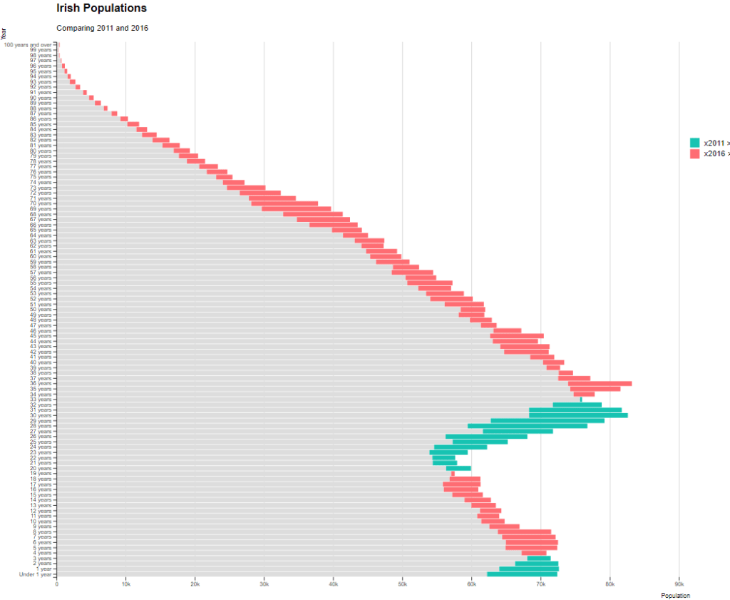 

We can see that under the age of four-ish, 2011 had more at the time. And again, there were people in their twenties in 2011 compared to 2016.

However, there are more older people in 2016 than in 2011.

Similar to above it is a bit busy! So we can create groups for every five age years categories and examine the broader trends with fewer horizontal bars.

First we want to remove the word “years” from the age variable and convert it to a numeric class variable. We can easily do this with the parse_number() function from the readr package

irish_wide %<>% 
mutate(age_num = readr::parse_number(as.character(age_last_birthday))) 

Next we can group the age years together into five year categories, zero to 5 years, 6 to 10 years et cetera.

We use the cut() function to divide the numeric age_num variable into equal groups. We use the seq() function and input age 0 to 100, in increments of 5.

irish_wide$age_group = cut(irish_wide$age_num, seq(0, 100, 5))

Next, we can use group_by() to calculate the sum of each population number in each five year category.

And finally, we use the distinct() function to remove the duplicated rows (i.e. we only want to keep the first row that gives us the five year category’s population count for each category.

irish_wide %<>% 
  group_by(age_group) %>% 
  mutate(five_year_2011 = sum(x2011)) %>% 
  mutate(five_year_2016 = sum(x2016)) %>% 
  distinct(five_year_2011, five_year_2016, .keep_all = TRUE)

Next plot the bar chart with the five year categories

compareBars(irish_wide, age_group, five_year_2011, five_year_2016, orientation = "horizontal",
              xLabel = "Population",
              yLabel = "Year",
              titleLabel = "Irish Populations",
              subtitleLabel = "Comparing 2011 and 2016",
              fontFamily = "Arial",
              compareVarFill1 = "#FE6D73",
              compareVarFill2 = "#17C3B2") 

irish_wide2 %>% 
  select(age_group, five_year_2011, five_year_2016) %>% 
  pivot_longer(!age_group,
             names_to = "year", 
             values_to = "pop_count",
             values_drop_na = TRUE) %>% 
  mutate(year = as.factor(year)) -> irishlong2

irishlong2 %>%   
  pyramid_chart(age_group, pop_count, year)