This blog will run through how to make a word cloud with Mill’s “On Liberty”, a treatise which argues that the state should never restrict people’s individual pursuits or choices (unless such choices harm others in society).
First, we install and load the gutenbergr package to access the catalogue of books from Project Gutenburg . This gutenberg_metadata function provides access to the website and its collection of around 60,000 digitised books in the public domain, for which their U.S. copyright has expired. This website is an amazing resource in its own right.
install.packages("gutenbergr")
library(gutenbergr)
Next we choose a book we want to download. We can search through the Gutenberg Project catalogue (with the help of the dplyr package). In the filter( ) function, we can search for a book in the library by supplying a string search term in “quotations”. Click here to see the CRAN package PDF. For example, we can look for all the books written by John Stuart Mill (search second name, first name) on the website:
mill_all <- gutenberg_metadata %>%
  filter(author = "Mill, John Stuart")
Or we can search for the title of the book:
mill_liberty <- gutenberg_metadata %>%
  filter(title = "On Liberty")
We now have a tibble of all the sentences in the book!
View(mill_liberty)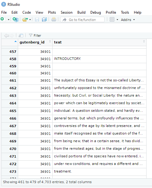
We see there are two variables in this new datafram and 4,703 string rows.
To extract every word as a unit, we need the unnest_tokens( ) function from the tidytext package:
install.packages("tidytext")
library(tidytext)
We take our mill_liberty object from above and indicate we want the unit to be words from the text. And we create a new mill_liberty_words object to hold the book in this format.
mill_liberty_words <- mill_liberty %>%
    unnest_tokens(word, text) %>%
    anti_join(stop_words)
We now have a row for each word, totalling to 17,576 words! This excludes words such as “the”, “of”, “to” and all those small sentence builder words.
Now we have every word from “On Liberty”, we can see what words appear most frequently! We can either create a list with the count( ) function:
count_word <- mill_liberty_words %>%
   count(word, sort = TRUE)
The default for a tibble object is printing off the first ten observations. If we want to see more, we can increase the n in our print argument.
print(liberty_words, n=30)
An alternative to this is making a word cloud to visualise the relative frequencies of these terms in the text.
For this, we need to install the wordcloud package.
install.packages("wordcloud")
library(wordcloud)
To get some nice colour palettes, we can also install the RColorBrewer package also:
install.packages("RColorBrewer")
library(RColorBrewer)
Check out the CRAN PDF on the wordcloud package to tailor your specifications.
For example, the rot.per argument indicates proportion words we want with 90 degree rotation. In my example, I have 30% of the words being vertical. I reran the code until the main one was horizontal, just so it pops out more.
With the scale option, we can indicate the range of the size of the words (for example from size 4 to size 0.5) in the example below
We can choose how many words we want to include in the wordcloud with the max.words argument
color_number <- 20
color_palette <- colorRampPalette(brewer.pal(8, "Paired"))(color_number)

wordcloud(words = mill_liberty_words$word, min.freq = 2,
 scale = c(4, 0.5)
          max.words=200, random.order=FALSE, rot.per=0.3,
          colors=color_palette)
We can see straightaway the most frequent word in the book is opinion. Given that this book forms one of the most rigorous defenses of the idea of freedom of speech, a free press and therefore against the a priori censorship of dissent in society, these words check out.
If we run the code with random.order=TRUE option, the cloud would look like this:
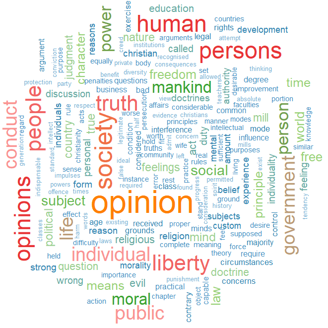
And you can play with proportions, colours, sizes and word placement until you find one you like!
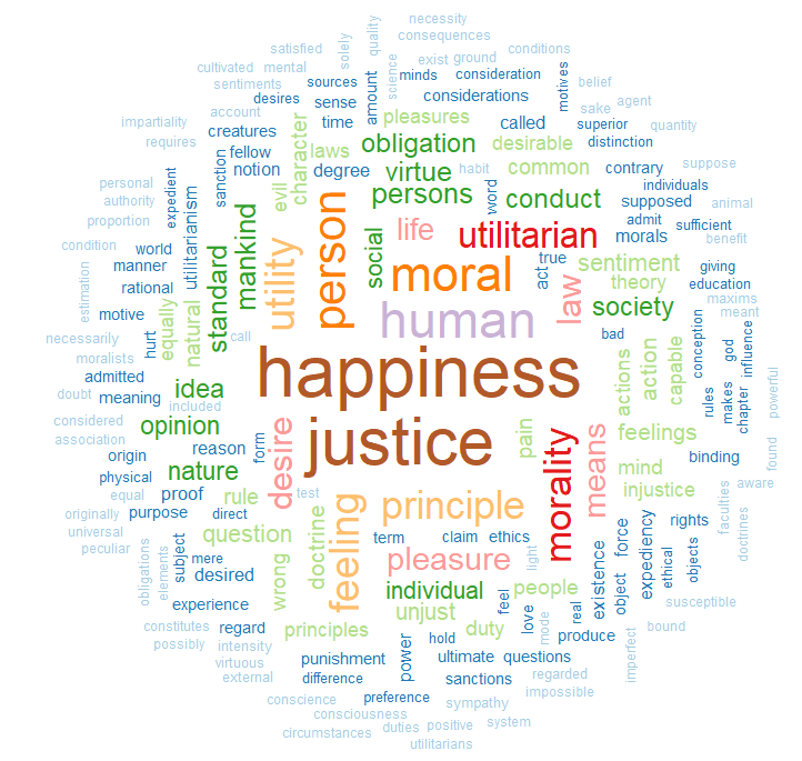
This word cloud highlights the most frequently used words in John Stuart Mill’s “Utilitarianism”: