Add weights to survey data with survey package in R: Part 2

Click here to read why need to add pspwght and pweight to the ESS data in Part 1.

Packages we will need:

library(survey)
library(srvy)
library(stargazer)
library(gtsummary)
library(tidyverse)

Click here to learn how to access and download ESS round data for the thirty-ish European countries (depending on the year).

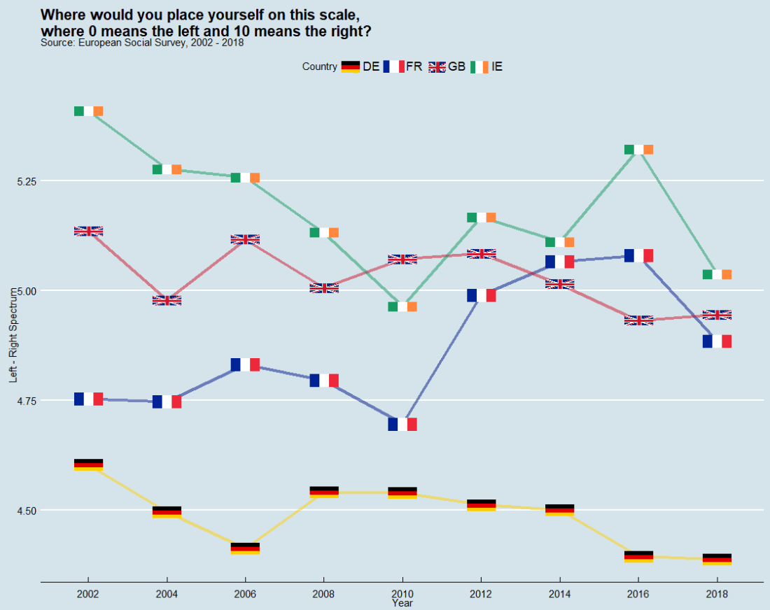
So with the essurvey package, I have downloaded and cleaned up the most recent round of the ESS survey, conducted in 2018.

We will examine the different demographic variables that relate to levels of trust in politicians across 29 European countries (education level, gender, age et cetera).

Before we create the survey weight objects, we can first make a bar chart to look at the different levels of trust in the different countries.

We can use the cut() function to divide the 10-point scale into three groups of “low”, “mid” and “high” levels of trust in politicians.

I also choose traffic light hex colors in color_palette vector and add full country names with countrycode() so it’s easier to read the graph

color_palette <- c("1" = "#f94144", "2" = "#f8961e", "3" = "#43aa8b")

round9$country_name <- countrycode(round9$country, "iso2c", "country.name")

trust_graph <- round9 %>% 
  dplyr::filter(!is.na(trust_pol)) %>% 
  dplyr::mutate(trust_category = cut(trust_pol, 
                                     breaks=c(-Inf, 3, 7, Inf), 
                                     labels=c(1,2,3))) %>% 
  mutate(trust_category = as.numeric(trust_category)) %>% 
  mutate(trust_pol_fac = as.factor(trust_category)) %>%
  ggplot(aes(x = reorder(country_name, trust_category))) +
  geom_bar(aes(fill = trust_pol_fac), 
               position = "fill") +
  bbplot::bbc_style() +
  coord_flip() 

trust_graph <- trust_graph + scale_fill_manual(values= color_palette, 
                                      name="Trust level",
                                      breaks=c(1,2,3),
                                      labels=c("Low", "Mid", "High")) 

The graph lists countries in descending order according to the percentage of sampled participants that indicated they had low trust levels in politicians.

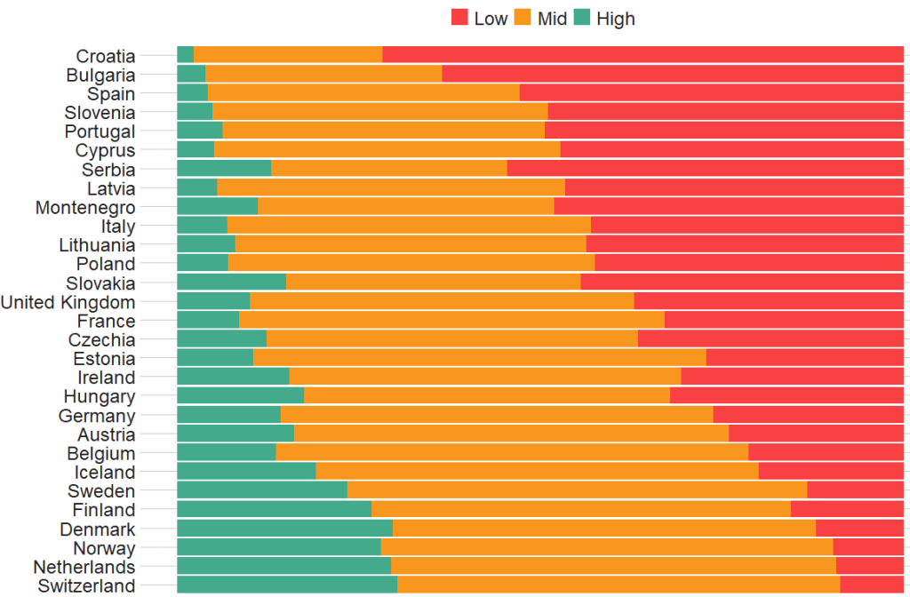
The respondents in Croatia, Bulgaria and Spain have the most distrust towards politicians.

For this example, I want to compare different analyses to see what impact different weights have on the coefficient estimates and standard errors in the regression analyses:

  • with no weights (dEfIniTelYy not recommended by ESS)
  • with post-stratification weights only (not recommended by ESS) and
  • with the combined post-strat AND population weight (the recommended weighting strategy according to ESS)

First we create two special svydesign objects, with the survey package. To create this, we need to add a squiggly ~ symbol in front of the variables (Google tells me it is called a tilde).

The ids argument takes the cluster ID for each participant.

psu is a numeric variable that indicates the primary sampling unit within which the respondent was selected to take part in the survey. For example in Ireland, this refers to the particular electoral division of each participant.

The strata argument takes the numeric variable that codes which stratum each individual is in, according to the type of sample design each country used.

The first svydesign object uses only post-stratification weights: pspwght

Finally we need to specify the nest argument as TRUE. I don’t know why but it throws an error message if we don’t …

post_design <- svydesign(ids = ~psu, 
                         strata = ~stratum, 
                         weights = ~pspwght
                         data = round9, 
                         nest = TRUE)

To combine the two weights, we can multiply them together and store them as full_weight. We can then use that in the svydesign function

r2$full_weight <- r2$pweight*r2$pspwght
 

full_design <- svydesign(ids = ~psu, 
                         strata = ~stratum, 
                         weights = ~full_weight,
                         data = round9, 
                         nest = TRUE)
class(full_design)

With the srvyr package, we can convert a “survey.design” class object into a “tbl_svy” class object, which we can then use with tidyverse functions.

full_tidy_design <- as_survey(full_design)
class(full_tidy_design)

Click here to read the CRAN PDF for the srvyr package.

We can first look at descriptive statistics and see if the values change because of the inclusion of the weighted survey data.

First, we can compare the means of the survey data with and without the weights.

We can use the gtsummary package, which creates tables with tidyverse commands. It also can take a survey object

library(gtsummary)
round9 %>% select(trust_pol, trust_pol, age, edu_years, gender, religious, left_right, rural_urban) %>% 
  tbl_summary(include = c(trust_pol, age, edu_years, gender, religious, left_right, rural_urban),
                 statistic = list(all_continuous() ~"{mean} ({sd})"))

And we look at the descriptive statistics with the full_design weights:

full_design %>% 
  tbl_svysummary(include = c(trust_pol, age, edu_years, gender, religious, left_right),
                 statistic = list(all_continuous() ~"{mean} ({sd})"))
WITHOUT weights AND WITH weights (post-stratification and population weights)

We can see that gender variable is more equally balanced between males (1) and females (2) in the data with weights

Additionally, average trust in politicians is lower in the sample with full weights.

Participants are more left-leaning on average in the sample with full weights than in the sample with no weights.

Next, we can look at a general linear model without survey weights and then with the two survey weights we just created.

Do we see any effect of the weighting design on the standard errors and significance values?

So, we first run a simple general linear model. In this model, R assumes that the data are independent of each other and based on that assumption, calculates coefficients and standard errors.

simple_glm <- glm(trust_pol ~ left_right + edu_years + rural_urban + age, data = round9)

Next, we will look at only post-stratification weights. We use the svyglm function and instead of using the data = r2, we use design = post_design .

post_strat_glm <- svyglm(trust_pol ~ left_right + edu_years + rural_urban  + age, design = post_design) 

And finally, we will run the regression with the combined post-stratification AND population weight with the design = full_design argument.

full_weight_glm <- svyglm(trust_pol ~ left_right + edu_years + rural_urban + age, design = full_design))

With the stargazer package, we can compare the models side-by-side:

library(stargazer)
stargazer(simple_glm, post_strat_glm, full_weight_glm, type = "text")

We can see that the standard errors in brackets were increased for most of the variables in model (3) with both weights when compared to the first model with no weights.

The biggest change is the rural-urban scale variable. With no weights, it is positive correlated with trust in politicians. That is to say, the more urban a location the respondent lives, the more likely the are to trust politicians. However, after we apply both weights, it becomes negative correlated with trust. It is in fact the more rural the location in which the respondent lives, the more trusting they are of politicians.

Additionally, age becomes statistically significant, after we apply weights.

Of course, this model is probably incorrect as I have assumed that all these variables have a simple linear relationship with trust levels. If I really wanted to build a robust demographic model, I would have to consult the existing academic literature and test to see if any of these variables are related to trust levels in a non-linear way. For example, it could be that there is a polynomial relationship between age and trust levels, for example. This model is purely for illustrative purposes only!

Plus, when I examine the R2 score for my models, it is very low; this model of demographic variables accounts for around 6% of variance in level of trust in politicians. Again, I would have to consult the body of research to find other explanatory variables that can account for more variance in my dependent variable of interest!

We can look at the R2 and VIF score of GLM with the summ() function from the jtools package. The summ() function can take a svyglm object. Click here to read more about various functions in the jtools package.

Sarcastic Nancy Pelosi GIF by MOODMAN - Find & Share on GIPHY
Advertisement

Add weights to survey data with survey package in R: Part 1

With the European Social Survey (ESS), we will examine the different variables that are related to levels of trust in politicians across Europe in the latest round 9 (conducted in 2018).

Click here for Part 2.

Click here to learn about downloading ESS data into R with the essurvey package.

Packages we will need:

library(survey)
library(srvyr)

The survey package was created by Thomas Lumley, a professor from Auckland. The srvyr package is a wrapper packages that allows us to use survey functions with tidyverse.

Why do we need to add weights to the data when we analyse surveys?

When we import our survey data file, R will assume the data are independent of each other and will analyse this survey data as if it were collected using simple random sampling.

However, the reality is that almost no surveys use a simple random sample to collect data (the one exception being Iceland in ESS!)

Excited Rachel Mcadams GIF by NETFLIX - Find & Share on GIPHY

Rather, survey institutions choose complex sampling designs to reduce the time and costs of ultimately getting responses from the public.

Their choice of sampling design can lead to different estimates and the standard errors of the sample they collect.

For example, the sampling weight may affect the sample estimate, and choice of stratification and/or clustering may mean (most likely underestimated) standard errors.

As a result, our analysis of the survey responses will be wrong and not representative to the population we want to understand. The most problematic result is that we would arrive at statistical significance, when in reality there is no significant relationship between our variables of interest.

Therefore it is essential we don’t skip this step of correcting to account for weighting / stratification / clustering and we can make our sample estimates and confidence intervals more reliable.

This table comes from round 8 of the ESS, carried out in 2016. Each of the 23 countries has an institution in charge of carrying out their own survey, but they must do so in a way that meets the ESS standard for scientifically sound survey design (See Table 1).

Sampling weights aim to capture and correct for the differing probabilities that a given individual will be selected and complete the ESS interview.

For example, the population of Lithuania is far smaller than the UK. So the probability of being selected to participate is higher for a random Lithuanian person than it is for a random British person.

Additionally, within each country, if the survey institution chooses households as a sampling element, rather than persons, this will mean that individuals living alone will have a higher probability of being chosen than people in households with many people.

Click here to read in detail the sampling process in each country from round 1 in 2002. For example, if we take my country – Ireland – we can see the many steps involved in the country’s three-stage probability sampling design.

St Patricks Day Snl GIF by Saturday Night Live - Find & Share on GIPHY

The Primary Sampling Unit (PSU) is electoral districts. The institute then takes addresses from the Irish Electoral Register. From each electoral district, around 20 addresses are chosen (based on how spread out they are from each other). This is the second stage of clustering. Finally, one person is randomly chosen in each house to answer the survey, chosen as the person who will have the next birthday (third cluster stage).

Click here for more information about Design Effects (DEFF) and click here to read how ESS calculates design effects.

DEFF p refers to the design effect due to unequal selection probabilities (e.g. a person is more likely to be chosen to participate if they live alone)

DEFF c refers to the design effect due to clustering

According to Gabler et al. (1999), if we multiply these together, we get the overall design effect. The Irish design that was chosen means that the data’s variance is 1.6 times as large as you would expect with simple random sampling design. This 1.6 design effects figure can then help to decide the optimal sample size for the number of survey participants needed to ensure more accurate standard errors.

So, we can use the functions from the survey package to account for these different probabilities of selection and correct for the biases they can cause to our analysis.

In this example, we will look at demographic variables that are related to levels of trust in politicians. But there are hundreds of variables to choose from in the ESS data.

Click here for a list of all the variables in the European Social Survey and in which rounds they were asked. Not all questions are asked every year and there are a bunch of country-specific questions.

We can look at the last few columns in the data.frame for some of Ireland respondents (since we’ve already looked at the sampling design method above).

The dweight is the design weight and it is essentially the inverse of the probability that person would be included in the survey.

The pspwght is the post-stratification weight and it takes into account the probability of an individual being sampled to answer the survey AND ALSO other factors such as non-response error and sampling error. This post-stratificiation weight can be considered a more sophisticated weight as it contains more additional information about the realities survey design.

The pweight is the population size weight and it is the same for everyone in the Irish population.

When we are considering the appropriate weights, we must know the type of analysis we are carrying out. Different types of analyses require different combinations of weights. According to the ESS weighting documentation:

  • when analysing data for one country alone – we only need the design weight or the poststratification weight.
  • when comparing data from two or more countries but without reference to statistics that combine data from more than one country – we only need the design weight or the poststratification weight
  • when comparing data of two or more countries and with reference to the average (or combined total) of those countries – we need BOTH design or post-stratification weight AND population size weights together.
  • when combining different countries to describe a group of countries or a region, such as “EU accession countries” or “EU member states” = we need BOTH design or post-stratification weights AND population size weights.

ESS warn that their survey design was not created to make statistically accurate region-level analysis, so they say to carry out this type of analysis with an abundance of caution about the results.

ESS has a table in their documentation that summarises the types of weights that are suitable for different types of analysis:

Since we are comparing the countries, the optimal weight is a combination of post-stratification weights AND population weights together.

Click here to read Part 2 and run the regression on the ESS data with the survey package weighting design

Below is the code I use to graph the differences in mean level of trust in politicians across the different countries.

library(ggimage) # to add flags
library(countrycode) # to add ISO country codes

# r_agg is the aggregated mean of political trust for each countries' respondents.

r_agg %>% 
  dplyr::mutate(country, EU_member = ifelse(country == "BE" | country == "BG" | country == "CZ" | country == "DK" | country == "DE" | country == "EE" | country == "IE" | country == "EL" | country == "ES" | country == "FR" | country == "HR" | country == "IT" | country == "CY" | country == "LV" | country == "LT" | country == "LU" | country == "HU" | country == "MT" | country == "NL" | country == "AT" | country == "AT" | country == "PL" | country == "PT" | country == "RO" | country == "SI" | country == "SK" | country == "FI" | country == "SE","EU member", "Non EU member")) -> r_agg


r_agg %>% 
  filter(EU_member == "EU member") %>% 
  dplyr::summarize(eu_average = mean(mean_trust_pol)) 


r_agg$country_name <- countrycode(r_agg$country, "iso2c", "country.name")


#eu_average <- r_agg %>%
 # summarise_if(is.numeric, mean, na.rm = TRUE)


eu_avg <- data.frame(country = "EU average",
                     mean_trust_pol = 3.55,
                     EU_member =  "EU average",
                     country_name = "EU average")

r_agg <- rbind(r_agg, eu_avg)

 
my_palette <- c("EU average" = "#ef476f", 
                "Non EU member" = "#06d6a0", 
                "EU member" = "#118ab2")

r_agg <- r_agg %>%          
  dplyr::mutate(ordered_country = fct_reorder(country, mean_trust_pol))


r_graph <- r_agg %>% 
  ggplot(aes(x = ordered_country, y = mean_trust_pol, group = country, fill = EU_member)) +
  geom_col() +
  ggimage::geom_flag(aes(y = -0.4, image = country), size = 0.04) +
  geom_text(aes(y = -0.15 , label = mean_trust_pol)) +
  scale_fill_manual(values = my_palette) + coord_flip()

r_graph 

Graph countries on the political left right spectrum

In this post, we can compare countries on the left – right political spectrum and graph the trends.

In the European Social Survey, they ask respondents to indicate where they place themselves on the political spectrum with this question: “In politics people sometimes talk of ‘left’ and ‘right’. Where would you place yourself on this scale, where 0 means the left and 10 means the right?”

Click here to read how to download data from the European Social survey.

round <- import_all_rounds()

Extract all the lists. I just want three of the variables for my graph.

r1 <- round[[1]]

r1 <- data.frame(country = r1$cntry, round= r1$essround, lrscale = r1$lrscale)

Do this for all the data.frames and rbind() them all together.

round_df <- rbind(r1, r2, r3, r4, r5, r6, r7, r8, r9)

Convert all the variables to suitable types:

round_df$country <- as.factor(round_df$country)
round_df$round <- as.numeric(round_df$round)
round_df$lrscale <- as.numeric(round_df$lrscale)

Next we find the mean score for all respondents in each of the countries for each year.

round_df %>% 
  dplyr::filter(!is.na(lrscale)) %>% 
  dplyr::group_by(country, round) %>% 
  dplyr::mutate(mean_lr = mean(lrscale)) -> round_df

We keep only one of the values for each country at each survey year.

round_df <- round_df[!duplicated(round_df$mean_lr),]

Create a vector of hex colors that correspond to the countries I want to look at: Ireland, France, the UK and Germany.

my_palette <- c( "DE" = "#FFCE00", "FR" = "#001489", "GB" = "#CF142B", "IE" = "#169B62")

And graph the plot:

library(ggthemes, ggimage)

lrscale_graph <- round_df %>% 
  dplyr::filter(country == "IE" | country == "GB" | country == "FR" | country == "DE") %>% 
  ggplot(aes(x= round, y = mean_lr, group = country)) +
  geom_line(aes(color = factor(country)), size = 1.5, alpha = 0.5) +
  ggimage::geom_flag(aes(image = country), size = 0.04) + 
  scale_color_manual(values = my_palette) +
  scale_x_discrete(name = "Year", limits=c("2002","2004","2006","2008","2010","2012","2014","2016","2018")) +
  labs(title = "Where would you place yourself on this scale,\n where 0 means the left and 10 means the right?",
       subtitle = "Source: European Social Survey, 2002 - 2018",
       fill="Country",
       x = "Year",
       y = "Left - Right Spectrum")

lrscale_graph + guides(color=guide_legend(title="Country")) + theme_economist()

Download European Social Survey data with essurvey package in R

The European Social Survey (ESS) measure attitudes in thirty-ish countries (depending on the year) across the European continent. It has been conducted every two years since 2001.

The survey consists of a core module and two or more ‘rotating’ modules, on social and public trust; political interest and participation; socio-political orientations; media use; moral, political and social values; social exclusion, national, ethnic and religious allegiances; well-being, health and security; demographics and socio-economics.

So lots of fun data for political scientists to look at.

install.packages("essurvey")
library(essurvey)

The very first thing you need to do before you can download any of the data is set your email address.

set_email("rforpoliticalscience@gmail.com")

Don’t forget the email address goes in as a string in “quotations marks”.

Show what countries are in the survey with the show_countries() function.

show_countries()
[1] "Albania"     "Austria"    "Belgium"           
[4] "Bulgaria"    "Croatia"     "Cyprus"            
[7] "Czechia"     "Denmark"     "Estonia"           
[10] "Finland"    "France"      "Germany"           
[13] "Greece"     "Hungary"     "Iceland"           
[16] "Ireland"    "Israel"      "Italy"             
[19] "Kosovo"     "Latvia"      "Lithuania"         
[22] "Luxembourg" "Montenegro"  "Netherlands"       
[25] "Norway"     "Poland"      "Portugal"          
[28] "Romania" "Russian Federation" "Serbia"            
[31] "Slovakia"   "Slovenia"     "Spain"             
[34] "Sweden"     "Switzerland"  "Turkey"            
[37] "Ukraine"    "United Kingdom"

It’s important to know that country names are case sensitive and you can only use the name printed out by show_countries(). For example, you need to write “Russian Federation” to access Russian survey data; if you write “Russia”…

Kamala Harris Reaction GIF by Markpain - Find & Share on GIPHY

Using these country names, we can download specific rounds or waves (i.e survey years) with import_country.  We have the option to choose the two most recent rounds, 8th (from 2016) and 9th round (from 2018).

ire_data <- import_all_cntrounds("Ireland")

The resulting data comes in the form of nine lists, one for each round

These rounds correspond to the following years:

  • ESS Round 9 – 2018
  • ESS Round 8 – 2016
  • ESS Round 7 – 2014
  • ESS Round 6 – 2012
  • ESS Round 5 – 2010
  • ESS Round 4 – 2008
  • ESS Round 3 – 2006
  • ESS Round 2 – 2004
  • ESS Round 1 – 2002

I want to compare the first round and most recent round to see if Irish people’s views have changed since 2002. In 2002, Ireland was in the middle of an economic boom that we called the “Celtic Tiger”. People did mad things like buy panini presses and second house in Bulgaria to resell. Then the 2008 financial crash hit the country very hard.

Irish people during the Celtic Tiger:

Music Video GIF - Find & Share on GIPHY

Irish people after the Celtic Tiger crash:

Big Cats GIF by NETFLIX - Find & Share on GIPHY

Ireland in 2018 was a very different place. So it will be interesting to see if these social changes translated into attitude changes.

First, we use the import_country() function to download data from ESS. Specify the country and rounds you want to download.

ire <-import_country(country = "Ireland", rounds = c(1, 9))

The resulting ire object is a list, so we’ll need to extract the two data.frames from the list:

ire_1 <- ire[[1]]

ire_9 <- ire[[2]]

The exact same questions are not asked every year in ESS; there are rotating modules, sometimes questions are added or dropped. So to merge round 1 and round 9, first we find the common columns with the intersect() function.

common_cols <- intersect(colnames(ire_1), colnames(ire_9))

And then bind subsets of the two data.frames together that have the same columns with rbind() function.

ire_df <- rbind(subset(ire_1, select = common_cols),
                subset(ire_9, select = common_cols))

Now with my merged data.frame, I only want to look at a few of the variables and clean up the dataset for the analysis.

Click here to look at all the variables in the different rounds of the survey.

att9 <- data.frame(country = data9$cntry,
                   round = data9$essround,
                   imm_same_eth = data9$imsmetn,
                   imm_diff_eth = data9$imdfetn,
                   imm_poor = data9$impcntr,
                   imm_econ = data9$imbgeco,
                   imm_culture = data9$imueclt,
                   imm_qual_life = data9$imwbcnt,
                   left_right = data9$lrscale)

class(att9$imm_same_eth)

All the variables in the dataset are a special class called “haven_labelled“. So we must convert them to numeric variables with a quick function. We exclude the first variable because we want to keep country name as a string character variable.

att_df[2:15] <- lapply(att_df[2:15], function(x) as.numeric(as.character(x)))

We can look at the distribution of our variables and count how many missing values there are with the skim() function from the skimr package

library(skimr)

skim(att_df)

We can run a quick t-test to compare the mean attitudes to immigrants on the statement: “Immigrants make country worse or better place to live” across the two survey rounds.

Lower scores indicate an attitude that immigrants undermine Ireland’ quality of life and higher scores indicate agreement that they enrich it!

t.test(att_df$imm_qual_life ~ att_df$round)

In future blog, I will look at converting the raw output of R into publishable tables.

The results of the independent-sample t-test show that if we compare Ireland in 2002 and Ireland in 2018, there has been a statistically significant increase in positive attitudes towards immigrants and belief that Ireland’s quality of life is more enriched by their presence in the country.

As I am currently an immigrant in a foreign country myself, I am glad to come from a country that sees the benefits of immigrants!

Donald Glover Yes GIF - Find & Share on GIPHY

If we load the ggpubr package, we can graphically look at the difference in mean attitude scores.

library(ggpubr)

box1 <- ggpubr::ggboxplot(att_df, x = "round", y = "imm_qual_life", color = "round", palette = c("#d11141", "#00aedb"),
 ylab = "Attitude", xlab = "Round")

box1 + stat_compare_means(method = "t.test")

It’s not the most glamorous graph but it conveys the shift in Ireland to more positive attitudes to immigration!

I suspect that a country’s economic growth correlates with attitudes to immigration.

So let’s take the mean annual score values

ire_agg <- ireland[!duplicated(ireland$mean_imm_qual_life),]
ire_agg <- ire_agg %>% 
select(year, everything())

Next we can take data from Quandl website on annual Irish GDP growth (click here to learn how to access economic data via a Quandl API on R.)

gdp <- Quandl('ODA/IRL_LE', start_date='2002-01-01', end_date='2020-01-01',type="raw")

Create a year variable from the date variable

gdp$year <- substr(gdp$Date, start = 1, stop = 4)

Add year variable to the ire_agg data.frame that correspond to the ESS survey rounds.

year =c("2002","2004","2006","2008","2010","2012","2014","2016","2018")
year <- data.frame(year)
ire_agg <- cbind(ire_agg, year)

Merge the GDP and ESS datasets

ire_agg <- merge(ire_agg, gdp, by.x = "year", by.y = "year", all.x = TRUE)

Scale the GDP and immigrant attitudes variables so we can put them on the same plot.

ire_agg$scaled_gdp <- scale(ire_agg$Value)

ire_agg$scaled_imm_attitude <- scale(ire_agg$mean_imm_qual_life)

In order to graph both variables on the same graph, we turn the two scaled variables into two factors of a single variable.

ire_agg <- ire_agg %>%
  select(year, scaled_imm_attitude, scaled_gdp) %>%
  gather(key = "variable", value = "value", -year)

Next, we can change the names of the factors

ire_agg$variable <- revalue(ire_agg$variable, c("scaled_gdp"="GDP (scaled)", "scaled_imm_attitude" = "Attitudes (scaled)"))

And finally, we can graph the plot.

The geom_rect() function graphs the coloured rectangles on the plot. I take colours from this color-hex website; the green rectangle for times of economic growth and red for times of recession. Makes sure the geom-rect() comes before the geom_line().

library(ggpthemes)

ggplot(ire_agg, aes(x = year, y = value, group = variable)) + geom_rect(aes(xmin= "2008",xmax= "2012",ymin=-Inf, ymax=Inf),fill="#d11141",colour=NA, alpha=0.01) +
  geom_rect(aes(xmin= "2002" ,xmax= "2008",ymin=-Inf, ymax=Inf),fill="#00b159",colour=NA, alpha=0.01) +
  geom_rect(aes(xmin= "2012" ,xmax= "2020",ymin=-Inf, ymax=Inf),fill="#00b159",colour=NA, alpha=0.01) +
  geom_line(aes(color = as.factor(variable), linetype = as.factor(variable)), size = 1.3) + 
  scale_color_manual(values = c("#00aedb", "#f37735")) + 
  geom_point() +
  geom_text(data=. %>%
              arrange(desc(year)) %>%
              group_by(variable) %>%
              slice(1), aes(label=variable), position= position_jitter(height = 0.3), vjust =0.3, hjust = 0.1, 
              size = 4, angle= 0) + ggtitle("Relationship between Immigration Attitudes and GDP Growth") + labs(value = " ") + xlab("Year") + ylab("scaled") + theme_hc()

And we can see that there is a relationship between attitudes to immigrants in Ireland and Irish GDP growth. When GDP is growing, Irish people see that immigrants improve quality of life in Ireland and vice versa. The red section of the graph corresponds to the financial crisis.