Cleaning up messy World Bank data

Packages we will need:

library(tidyverse)
library(tidyr)
library(janitor)
library(magrittr)
library(democracyData)
library(countrycode)
library(ggimage)

When you come across data from the World Bank, often it is messy.

So this blog will go through how to make it more tidy and more manageable in R

For this blog, we will look at World Bank data on financial aid. Specifically, we will be using values for net ODA received as percentage of each country’s GNI. These figures come from the Development Assistance Committee of the Organisation for Economic Co-operation and Development (DAC OECD).

If we look at the World Bank data downloaded from the website, we have a column for each year and the names are quite messy.

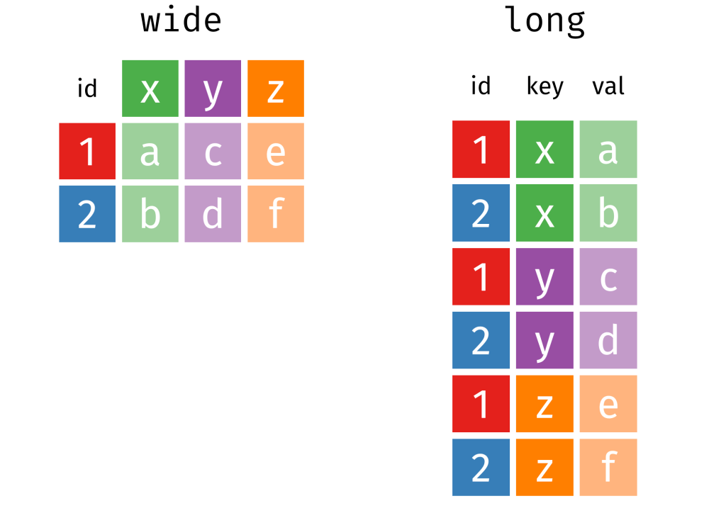
This data is wide form.

Unacceptable.

So we will change the data from wide to long data.

Instead of a column for each year, we will have a row for each country-year.

Before doing that, we can clean up the variable names with the janitor package function: clean_names().

sdg %<>% 
  clean_names() 

ALSO, before we pivot the dataset to longer format, we choose the variables we want to keep (i.e. only country, year and ODA value)

sdg %<>% 
  select(country_name, x1990_yr1990:x2015_yr2015) 

Now we are ready to turn the data from wide to long.

We can use the pivot_longer() function from the tidyr package.

Instead of 286 rows and 27 columns, we will ultimately end up with 6968 rows and only 3 columns.

Thank you to Mr. Aden-Buie for your page visualising all the different ways to transform datasets with dplyr. Click the link to check out more.

Back to the pivoting, we want to create a row for each year, 1990, 1991, 1992 …. up to 2015

And we will have a separate cell for each value of the ODA variable for each country-year value.

In the pivot_longer() function we exclude the country names,

We want a new row for each year, so we make a “year” variable with the names_to() argument.

And we create a separate value for each ODA as a percentage of GNI with the values_to() argument.

sdg %>% 
  pivot_longer(!country_name, names_to = "year", 
               values_to = "oda_gni") -> oda

The year values are character strings, not numbers. So we will convert with parse_number(). This parses the first number it finds, dropping any non-numeric characters before the first number and all characters after the first number.

oda %>% 
     mutate(year = parse_number(year)) -> oda 

Next we will move from the year variable to ODA variable. There are many ODA values that are empty. We can see that there are 145 instances of empty character strings.

oda %>% 
  count(oda_gni) %>% 
  arrange(oda_gni)

So we can replace the empty character strings with NA values using the na_if() function. Then we can use the parse_number() function to turn the character into a string.

oda %>%
  mutate(oda_gni = na_if(oda_gni, "")) %>% 
  mutate(oda_gni = parse_number(oda_gni)) -> oda

Now we need to delete the year variables that have no values.

oda %<>% 
  filter(!is.na(year))

Also we need to delete non-countries.

The dataset has lots of values for regions that are not actual countries. If you only want to look at politically sovereign countries, we can filter out countries that do not have a Correlates of War value.

oda %<>%
  mutate(cow = countrycode(oda$country_name, "country.name", 'cown')) %>% 
  filter(!is.na(cow))

We can also make a variable for each decade (1990s, 2000s etc).

oda %>% 
  mutate(decade = substr(year, 1, 3)) %>% 
  mutate(decade = paste0(decade, "0s"))

And download data for countries’ region, continent and govenment regime. To do this we use the democracyData package and download the PACL dataset.

Click here to read more about this package.

Download democracy data with democracyData package in R

pacl <- democracyData::redownload_pacl()

pacl %>% 
  select(cow = pacl_cowcode,
         year,
         region = un_region_name,
         continent = un_continent_name,
         demo_dummy = democracy,
         regime = regime
         ) -> pacl_subset

We use the left_join() function to join both datasets together with Correlates of War code and year variables.

oda %>% 
  left_join(pacl_subset, by = c("cow", "year")) -> oda_pacl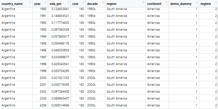

Now if we look at the dataset, we can see that it is much tidier and we can start analysing.

Below we can create a bar chart of the top ten countries that received the most aid as a percentage of their economic income (gross national income)

First we need to get the average oda per country with the group_by() and summarise() functions

oda_pacl %>%
  mutate(oda_gni = ifelse(is.na(oda_gni), 0, oda_gni)) %>%  
  group_by(country_name,region, continent) %>% 
  summarise(avg_oda = mean(oda_gni, na.rm = TRUE)) -> oda_mean

We use the slice() function to only have the top ten countries

oda_mean %>% 
  arrange(desc(avg_oda)) %>%
  ungroup() %>% 
  slice(1:10) -> oda_slice

We add an ISO code for each country for the flags

Click here to read more about the ggimage package

Add rectangular flags to graphs with ggimage package in R

oda_slice %<>% 
  mutate(iso2 = countrycode(country_name, "country.name", "iso2c"))

And some nice hex colours

my_palette <- c( "#44bec7", "#ffc300", "#fa3c4c")

And finally, plot it out with ggplot()

oda_slice %>%
  ggplot(aes(x = reorder(country_name, avg_oda),
             y = avg_oda, fill = continent)) + 
  geom_bar(stat = "identity") + 
  ggimage::geom_flag(aes(image = iso2), size = 0.1)  +
  coord_flip() +
  scale_fill_manual(values = my_palette) + 
  labs(title = "ODA aid as % GNI ",
       subtitle = "Source: OECD DAC via World Bank",
       x = "Donor Country",
       y = "ODA per capita") + bbplot::bbc_style()