How to download OECD datasets in R

Packages we will need:

library(OECD)
library(tidyverse)
library(magrittr)
library(janitor)
library(devtools)
library(readxl)
library(countrycode)
library(scales)
library(ggflags)
library(bbplot)

In this blog post, we are going to look at downloading data from the OECD statsitics and data website.

The Organisation for Economic Co-operation and Development (OECD) provides analysis, and policy recommendations for 38 industrialised countries.

Angry Work GIF by Jess - Find & Share on GIPHY

The 38 countries in the OECD are:

  • Australia
  • Austria
  • Belgium
  • Canada
  • Chile
  • Colombia
  • Czech Republic
  • Denmark
  • Estonia
  • Finland
  • France
  • Germany
  • Hungary
  • Iceland
  • Ireland
  • Israel
  • Italy
  • Japan
  • South Korea
  • Latvia
  • Lithuania
  • Luxembourg
  • Mexico
  • Netherland
  • New Zealand
  • Norway
  • Poland
  • Portugal
  • Slovakia
  • Slovenia
  • Spain
  • Sweden
  • Switzerland
  • Turkey
  • United Kingdom
  • United States
  • European Union

We can download the OCED data package directly from the github repository with install_github()

install_github("expersso/OECD")
library(OECD)

The most comprehensive tutorial for the package comes from this github page. Mostly, it gives a fair bit more information about filtering data

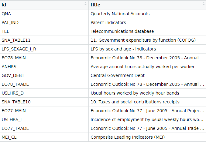
We can look at the all the datasets that we can download from the website via the package with the following get_datasets() function:
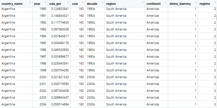
titles <- OECD::get_datasets()

This gives us a data.frame with the ID and title for all the OECD datasets we can download into the R console, as we can see below.

In total there are 1662 datasets that we can download.

These datasets all have different variable types, countries, year spans and measurement values. So it is important to check each dataset carefully when we download them.

We can filter key phrases to subset datasets:

 titles %>%  
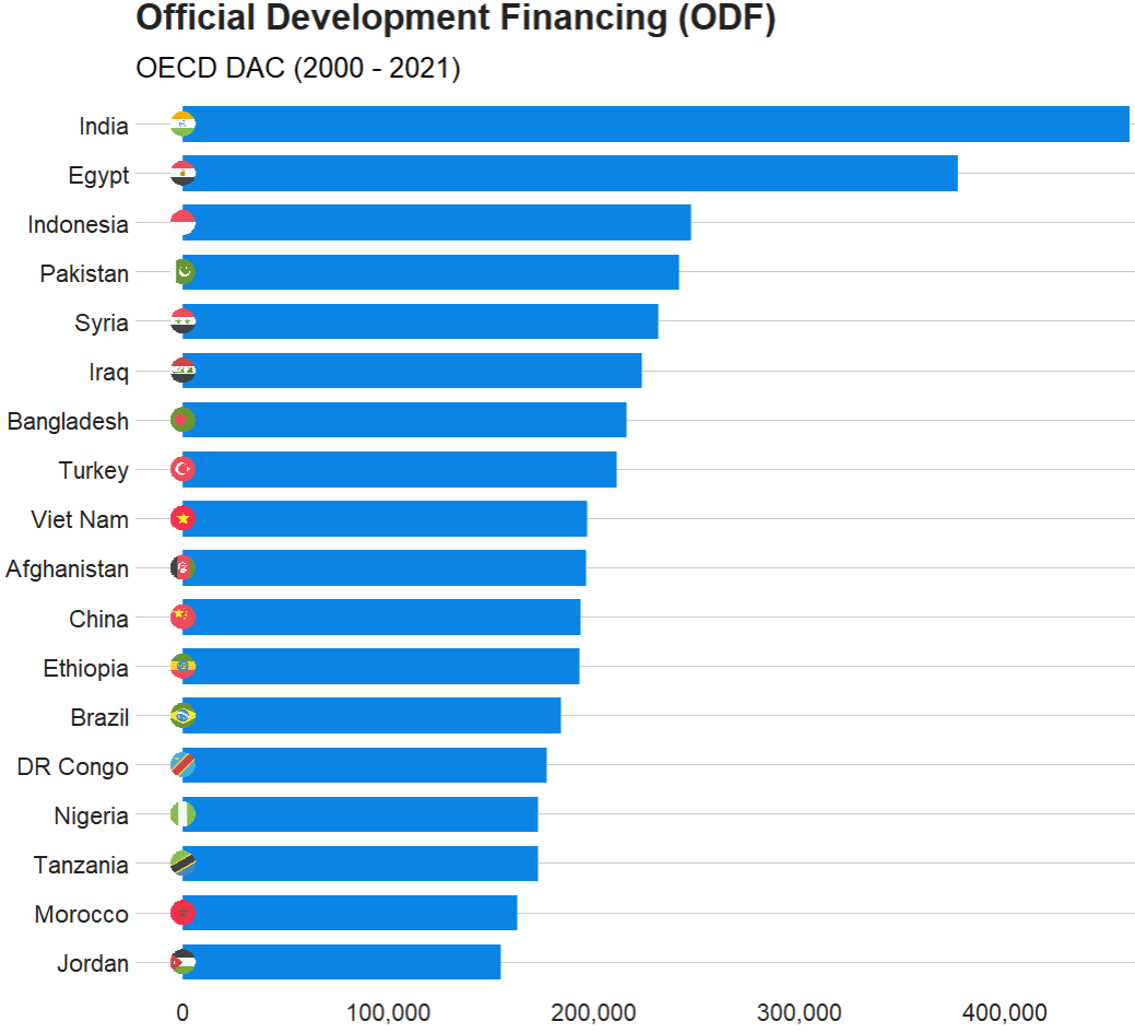
         filter(grepl("oda", title, ignore.case = TRUE)) %>% View

In this blog, we will graph out the Official Development Financing (ODF) for each country.

Official Development Financing measures the sum of RECEIVED (NOT DONATED) aid such as:

  • bilateral ODA aid
  • concessional and non-concessional resources from multilateral sources
  • bilateral other official flows made available for reasons unrelated to trade

Before we can charge into downloading any dataset, it is best to check out the variables it has. We can do that with the get_data_structure() function:

get_data_structure("REF_TOTAL_ODF") %>% 
       str(., max.level = 2)
 $ VAR_DESC       :'data.frame':	10 obs. of  2 variables:
  ..$ id         : chr [1:10] "RECIPIENT" "PART" "AMOUNTTYPE" "TIME" ...
  ..$ description: chr [1:10] "Recipient" "Part" "Amount type" "Year" ...

 $ RECIPIENT      :'data.frame':	301 obs. of  2 variables:
  ..$ id   : chr [1:301] "10200" "10100" "10010" "71" ...
  ..$ label: chr [1:301] "All Recipients, Total" "Developing Countries, Total" "Europe, Total" "Albania" ...

 $ PART           :'data.frame':	2 obs. of  2 variables:
  ..$ id   : chr [1:2] "1" "2"
  ..$ label: chr [1:2] "1 : Part I - Developing Countries" "2 : Part II - Countries in Transition"

 $ AMOUNTTYPE     :'data.frame':	2 obs. of  2 variables:
  ..$ id   : chr [1:2] "A" "D"
  ..$ label: chr [1:2] "Current Prices" "Constant Prices"

 $ TIME           :'data.frame':	62 obs. of  2 variables:
  ..$ id   : chr [1:62] "1960" "1961" "1962" "1963" ...
  ..$ label: chr [1:62] "1960" "1961" "1962" "1963" ...

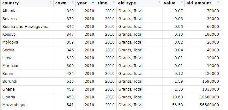
We will clean up the ODF dataset with the clean_names() function from janitor package.

aid <- get_dataset("REF_TOTAL_ODF")  %>% 
  janitor::clean_names()  %>%
  select(recipient, aid = obs_value, time)

One problem with this dataset is that we only have the DAC country codes in this dataset.

We will need to read in and merge the country code variables into the aid dataset.

dac_code <- readxl::read_excel(file.choose())

We can then clean up the DAC codes to merge with the aid data.

dac_code %<>%
    janitor::clean_names()  %>% 
    mutate(cown = countrycode(recipient_name_e, "country.name", "cown")) %>% 
    select(recipient_code,
         year, 
         cown,
         country = recipient_name_e,
         group_id, 
         dev_group = group_name_e,
         p_group = group_name_f,
         wb_group)

And merge with left_join()

aid %<>% 
  mutate(recipient_code = parse_number(recipient)) %>%  
  left_join(dac_code, by = c("recipient_code" = "recipient_code")) 

Next we can sum up the aid that each country received since 2000.

aid %>% 
  filter(year > 1999) %>%  
  filter(!is.na(country)) %>% 
  mutate(aid = parse_number(aid)) %>% 
  mutate(country = case_when(country == "Syrian Arab Republic" ~ "Syria", 
                             country == "T?rkiye" ~ "Turkey",
                             country == "China (People's Republic of)" ~ "China",
                             country == "Democratic Republic of the Congo" ~ "DR Congo",
                             TRUE ~ as.character(country))) %>% 
  group_by(country) %>% 
  summarise(total_aid = sum(aid, na.rm = TRUE)) %>% 
  ungroup() %>% 
  mutate(iso2 = tolower(countrycode(country, "country.name", "iso2c"))) %>% 
  filter(total_aid > 150000) %>% 
  ggplot(aes(x = reorder(country, total_aid),
             y = total_aid)) + 
  geom_bar(stat = "identity", 
           width = 0.7, 
           color = "#0a85e5", 
           fill = "#0a85e5") +
  ggflags::geom_flag(aes(x = country, y = -1, country = iso2), size = 8) +
  bbplot::bbc_style() + 
  scale_y_continuous(labels = scales::comma_format()) +
  coord_flip() + 
  labs(x = "ODA received", y = "", title = "Official Development Financing (ODF)", subtitle = "OECD DAC (2000 - 2021)")

The TIME_FORMAT can be any of the following types:

  • ‘P1Y’ for annual
  • ‘P6M’ for bi-annual
  • ‘P3M’ for quarterly
  • ‘P1M’ for monthly data.

To access each countries in the datasets, we can use the following codes

oecd_ios3 <- c("AUS", "AUT", "BEL", "CAN", "CHL", "COL", "CZE",
               "DNK", "EST", "FIN", "FRA", "DEU", "GRC", "HUN",
               "ISL", "IRL", "ISR", "ITA", "JPN", "KOR", "LVA", 
               "LTU", "LUX", "MEX", "NLD", "NZL", "NOR", "POL",
               "PRT", "SVK", "SVN", "ESP", "SWE", "CHE", "TUR",
               "GBR", "USA")

Alternatively, we can use only the EU countries that are in the OECD.

eu_oecd_iso3 <- c("AUT", "BEL", "CZE", "DNK", "EST", "FIN", 
                  "FRA", "DEU", "GRC", "HUN", "IRL", "ITA",
                  "LVA", "LTU", "LUX", "NLD", "POL", "PRT",
                  "SVK", "SVN", "ESP", "SWE")
sal_raw %>% 
  janitor::clean_names() %>% 
  filter(age == "Y25T64") %>% 
  filter(grade == "TE") %>% 
  filter(indicator == "NAT_ACTL_YR") %>% 
  filter(isc11 == "L1") %>% 
  filter(sex == "T") %>% 
  select(country, year = time, obs_value) -> sal
Advertisement

Cleaning up messy World Bank data

Packages we will need:

library(tidyverse)
library(tidyr)
library(janitor)
library(magrittr)
library(democracyData)
library(countrycode)
library(ggimage)

When you come across data from the World Bank, often it is messy.

So this blog will go through how to make it more tidy and more manageable in R

For this blog, we will look at World Bank data on financial aid. Specifically, we will be using values for net ODA received as percentage of each country’s GNI. These figures come from the Development Assistance Committee of the Organisation for Economic Co-operation and Development (DAC OECD).

If we look at the World Bank data downloaded from the website, we have a column for each year and the names are quite messy.

This data is wide form.

Unacceptable.

So we will change the data from wide to long data.

Instead of a column for each year, we will have a row for each country-year.

Before doing that, we can clean up the variable names with the janitor package function: clean_names().

sdg %<>% 
  clean_names() 

ALSO, before we pivot the dataset to longer format, we choose the variables we want to keep (i.e. only country, year and ODA value)

sdg %<>% 
  select(country_name, x1990_yr1990:x2015_yr2015) 

Now we are ready to turn the data from wide to long.

We can use the pivot_longer() function from the tidyr package.

Instead of 286 rows and 27 columns, we will ultimately end up with 6968 rows and only 3 columns.

Source: Garrick Aden-Buie’s (@grrrckTidy Animated Verbs

Thank you to Mr. Aden-Buie for your page visualising all the different ways to transform datasets with dplyr. Click the link to check out more.

Back to the pivoting, we want to create a row for each year, 1990, 1991, 1992 …. up to 2015

And we will have a separate cell for each value of the ODA variable for each country-year value.

In the pivot_longer() function we exclude the country names,

We want a new row for each year, so we make a “year” variable with the names_to() argument.

And we create a separate value for each ODA as a percentage of GNI with the values_to() argument.

sdg %>% 
  pivot_longer(!country_name, names_to = "year", 
               values_to = "oda_gni") -> oda

The year values are character strings, not numbers. So we will convert with parse_number(). This parses the first number it finds, dropping any non-numeric characters before the first number and all characters after the first number.

oda %>% 
     mutate(year = parse_number(year)) -> oda 

Next we will move from the year variable to ODA variable. There are many ODA values that are empty. We can see that there are 145 instances of empty character strings.

oda %>% 
  count(oda_gni) %>% 
  arrange(oda_gni)

So we can replace the empty character strings with NA values using the na_if() function. Then we can use the parse_number() function to turn the character into a string.

oda %>%
  mutate(oda_gni = na_if(oda_gni, "")) %>% 
  mutate(oda_gni = parse_number(oda_gni)) -> oda

Now we need to delete the year variables that have no values.

oda %<>% 
  filter(!is.na(year))

Also we need to delete non-countries.

The dataset has lots of values for regions that are not actual countries. If you only want to look at politically sovereign countries, we can filter out countries that do not have a Correlates of War value.

oda %<>%
  mutate(cow = countrycode(oda$country_name, "country.name", 'cown')) %>% 
  filter(!is.na(cow))

We can also make a variable for each decade (1990s, 2000s etc).

oda %>% 
  mutate(decade = substr(year, 1, 3)) %>% 
  mutate(decade = paste0(decade, "0s"))

And download data for countries’ region, continent and govenment regime. To do this we use the democracyData package and download the PACL dataset.

Click here to read more about this package.

pacl <- democracyData::redownload_pacl()

pacl %>% 
  select(cow = pacl_cowcode,
         year,
         region = un_region_name,
         continent = un_continent_name,
         demo_dummy = democracy,
         regime = regime
         ) -> pacl_subset

We use the left_join() function to join both datasets together with Correlates of War code and year variables.

oda %>% 
  left_join(pacl_subset, by = c("cow", "year")) -> oda_pacl

Now if we look at the dataset, we can see that it is much tidier and we can start analysing.

Below we can create a bar chart of the top ten countries that received the most aid as a percentage of their economic income (gross national income)

First we need to get the average oda per country with the group_by() and summarise() functions

oda_pacl %>%
  mutate(oda_gni = ifelse(is.na(oda_gni), 0, oda_gni)) %>%  
  group_by(country_name,region, continent) %>% 
  summarise(avg_oda = mean(oda_gni, na.rm = TRUE)) -> oda_mean

We use the slice() function to only have the top ten countries

oda_mean %>% 
  arrange(desc(avg_oda)) %>%
  ungroup() %>% 
  slice(1:10) -> oda_slice

We add an ISO code for each country for the flags

Click here to read more about the ggimage package

oda_slice %<>% 
  mutate(iso2 = countrycode(country_name, "country.name", "iso2c"))

And some nice hex colours

my_palette <- c( "#44bec7", "#ffc300", "#fa3c4c")

And finally, plot it out with ggplot()

oda_slice %>%
  ggplot(aes(x = reorder(country_name, avg_oda),
             y = avg_oda, fill = continent)) + 
  geom_bar(stat = "identity") + 
  ggimage::geom_flag(aes(image = iso2), size = 0.1)  +
  coord_flip() +
  scale_fill_manual(values = my_palette) + 
  labs(title = "ODA aid as % GNI ",
       subtitle = "Source: OECD DAC via World Bank",
       x = "Donor Country",
       y = "ODA per capita") + bbplot::bbc_style()

Examining Ireland’s foreign policy in pictures with R

Packages we will need:

library(peacesciencer)  
library(forcats)
library(ggflags)
library(tidyverse)
library(magrittr)
library(waffle)
library(bbplot)
library(rvest)

In January 2015, the Irish government published a review of Ireland’s foreign policy. The document, The Global Island: Ireland’s Foreign Policy for a Changing World offers a perspective on Ireland’s place in the world.

In this blog, we will graph out some of the key features of Ireland’ foreign policy and so we can have a quick overview of the key relationships and trends.

Excited Season 4 GIF by The Office - Find & Share on GIPHY

First, we will look at the aid that Ireland gives to foreign countries. This read.csv(file.choose()) will open up the file window and you can navigate to the file and data that you can download from DAC OECD website: https://data.oecd.org/oda/net-oda.htm

dac <- read.csv(file.choose())

We will filter only Ireland and clean the names with the clean_names() function from the janitor package:

dac %<>% 
  filter(Donor == "Ireland") %>% 
  clean_names()

And change the variables, adding the Correlates of War codes and cleaning up some of the countries’ names.

dac %<>% 
  mutate(cown = countrycode(recipient_2, "country.name", "cown"),
         aid_amount = value*1000000) %>%  
  select(country = recipient_2, cown,
         year, time, aid_type, value, aid_amount) %>%
  mutate(cown = ifelse(country == "West Bank and Gaza Strip", 6666,
         ifelse(country == "Serbia", 345, 
         ifelse(country == "Micronesia", 987,cown))))%>%
  filter(!is.na(cown)) 

Next we can convert dataframe to wider format so we have a value column for each aid type

dac %>% 
  distinct(country, cown, year, time, aid_type, value, .keep_all = TRUE)  %>%  
  pivot_wider(names_from = "aid_type", values_from = "aid_amount") %>% 
  mutate(across(where(is.numeric), ~ replace_na(., 0))) %>% 
  clean_names() -> dac_wider

And we graph out the three main types of aid:

dac_wider %>%
  group_by(year) %>% 
  summarise(total_humanitarian = sum(humanitarian_aid, na.rm = TRUE),
  total_technical = sum(technical_cooperation, na.rm = TRUE),
  total_development_food_aid = sum(development_food_aid)) %>% 
  ungroup() %>% 
  pivot_longer(!year, names_to = "aid_type", values_to = "aid_value") %>% 
  ggplot(aes(x = year, y = aid_value, groups = aid_type)) + 
  geom_line(aes(color = aid_type), size = 2, show_guide  = FALSE) +
  geom_point(aes(color = aid_type), fill = "white", shape = 21, size = 3, stroke = 2) +
  bbplot::bbc_style()  +
  scale_y_continuous(labels = scales::comma) + 
  scale_x_discrete(limits = c(2010:2018)) +
  labs(title = "Irish foreign aid by aid type (2010 - 2018)",
       subtitle = ("Source: OECD DAC")) +
  scale_color_discrete(name = "Aid type", 
        labels = c("Development and Food", "Humanitarian", "Technical"))

We will look at total ODA aid:

dac %>% 
  count(aid_type) %>% 
  arrange(desc(n)) %>% 
  knitr::kable(format = "html")
aid_type n
Imputed Multilateral ODA 2298
Memo: ODA Total, excl. Debt 1292
Memo: ODA Total, Gross disbursements 1254
ODA: Total Net 1249
Grants, Total 1203
Technical Cooperation 541
ODA per Capita 532
Humanitarian Aid 518
ODA as % GNI (Recipient) 504
Development Food Aid 9

And get some pretty hex colours:

pal_10 <- c("#001219","#005f73","#0a9396","#94d2bd","#e9d8a6","#ee9b00","#ca6702","#bb3e03","#ae2012","#9b2226")

And download some regime, democracy, region and continent data from the PACL datase with the democracyData() package

pacl <- redownload_pacl() 

pacl %<>% 
  mutate(regime_name = ifelse(regime == 0, "Parliamentary democracies",
         ifelse(regime == 1, "Mixed democracies",
         ifelse(regime == 2, "Presidential democracies",
         ifelse(regime == 3, "Civilian autocracies",
         ifelse(regime == 4, "Military dictatorships",
         ifelse(regime ==  5,"Royal dictatorships", regime))))))) %>%
  mutate(regime = as.factor(regime)) 

pacl %<>% 
  select(year, country = pacl_country, 
         democracy, regime_name,
         region_name = un_region_name, 
         continent_name = un_continent_name)

pacl %<>% 
  mutate(cown = countrycode(country, "country.name", "cown")) %>% 
  select(!country)

Summarise the total aid for each country across the years and choose the top 20 countries

dac %>% 
  filter(aid_type == "Memo: ODA Total, Gross disbursements") %>% 
  group_by(country) %>% 
  summarise(total_country_aid = sum(aid_amount, na.rm = TRUE)) %>% 
  ungroup() %>% 
  top_n(n = 20) %>% 
  mutate(cown = countrycode::countrycode(country, "country.name", "cown")) %>% 
  inner_join(pacl, by = "cown") %>%  
  mutate(region_name = ifelse(country == "West Bank and Gaza Strip", "Western Asia", region_name)) %>% 
  mutate(region_name = ifelse(region_name == "Western Asia", "Middle East", region_name)) %>% 
  mutate(country = ifelse(country == "West Bank and Gaza Strip", "Palestine",
  ifelse(country == "Democratic Republic of the Congo", "DR Congo",
  ifelse(country == "Syrian Arab Republic", "Syria", country)))) %>% 
  mutate(iso2 = tolower(countrycode::countrycode(country, "country.name", "iso2c"))) %>% 
  ggplot(aes(x = forcats::fct_reorder(country, total_country_aid), y = total_country_aid)) + 
  geom_bar(aes(fill = region_name), stat = "identity", width = 0.7) + 
  coord_flip() + bbplot::bbc_style() + 
  geom_flag(aes(x = country, y = -100, country = iso2), size = 12) +
  scale_fill_manual(values = pal_10) +
  labs(title = "Ireland's largest ODA foreign aid recipients, 2010 - 2018",
       subtitle = ("Source: OECD DAC")) + 
  xlab("") + ylab("") + 
  scale_x_continuous(labels = scales::comma)

We can make a waffle plot to look at the different types of regimes to which the Irish government gave aid over the decades

 dac %>% 
  mutate(decade = substr(year, 1, 3)) %>% 
  mutate(decade = paste0(decade, "0s")) %>% 
  group_by(decade) %>% 
  count(regime_name) %>% 
  ggplot(aes(fill = regime_name, values = n)) +
  geom_waffle(color = "white", size = 0.3, n_rows = 10, flip = TRUE) +
  facet_wrap(~decade, nrow = 1, strip.position = "bottom") + 
  bbplot::bbc_style()  +
  scale_fill_manual(values = pal_10) +
   scale_x_discrete(breaks = round(seq(0, 1, by = 0.2),3)) +
  labs(title = "Ireland's ODA foreign aid recipient regime types since 1945",
       subtitle = ("Source: OECD DAC"))  

Next, we will download dyadic foreign policy similarity measures from peacesciencer.

Peacesciencer package has tools and data sets for the study of quantitative peace science. 

Click here to read more about the peacesciencer package by Steven Miller

fp_similar_df <- peacesciencer::create_dyadyears() %>% 
  add_gwcode_to_cow() %>% 
  add_fpsim()	

I am only looking at dyadic foreign policy similarity with Ireland, so filter by Ireland’s Correlates of War code, 205.

Click here to find out all countries’ COW code

fp_similar_df %<>% 
  filter(ccode1 == 205)

Data on alliance portfolios comes from the Correlates of War and is used to calculate similarity of foreign policy positions (see Altfeld & Mesquita, 1979).

The assumption is that similar alliance portfolios are the result of similar foreign policy positions.

With increasing in level of commitment, the strength of alliance commitments can be:

  1. no commitment
  2. entente
  3. neutrality or nonaggression pact
  4. defense pact

We will map out alliance similarity. This will use the measurement calculated with Cohen’s Kappa. Check out Hage’s (2011) article to read more about the different ways to measure alliance similarity.

Next we can look at UN similarity.

The UN voting variable calculates three values:

1 = Yes

2 = Abstain

3 = No

Based on these data, if two countries in a similar way on the same UN resolutions, this is a measure of the degree to which dyad members’ foreign policy positions are similar.

fp_similarity_df %>% 
  mutate(country = countrycode::countrycode(ccode2, "cown", "country.name")) %>% 
  select(country, ccode2, year,
         un_similar = kappavv) %>% 
  filter(year > 1989) %>% 
  filter(!is.na(country)) %>%
  mutate(iso2 = tolower(countrycode::countrycode(country, "country.name", "iso2c"))) %>% 
  group_by(country) %>% 
  mutate(avg_un = mean(un_similar, na.rm = TRUE)) %>%
  distinct(country, avg_un, iso2, .keep_all = FALSE) %>% 
  ungroup() %>% 
  top_n(n = 10)  -> top_un_similar

And graph out the top ten

  top_un_similar %>%
  ggplot(aes(x = forcats::fct_reorder(country, avg_un), 
             y = avg_un)) + 
  geom_bar(stat = "identity",
           width = 0.7, 
           color = "#0a85e5", 
           fill = "#0a85e5") +
  ggflags::geom_flag(aes(x = country, y = 0, country = iso2), size = 15) +
  coord_flip() + bbplot::bbc_style()  +
  ggtitle("UN voting similarity with Ireland since 1990")

If we change the top_n() to negative, we can get the bottom 10

top_n(n = -10)

We can quickly scrape data about the EU countries with the rvest package


eu_members_html <- read_html("https://en.wikipedia.org/wiki/European_Union")
eu_members_tables <- eu_members_html %>% html_table(header = TRUE, fill = TRUE)

eu_member <- eu_members_tables[[6]]

eu_member %<>% 
  janitor::clean_names()

eu_member %>% distinct(state) %>%  pull(state) -> eu_state

Last we are going to look at globalization scores. The data comes from the the KOF Globalisation Index. This measures the economic, social and political dimensions of globalisation. Globalisation in the economic, social and political fields has been on the rise since the 1970s, receiving a particular boost after the end of the Cold War.

Click here for data that you can download comes from the KOF website

kof %>%
  filter(country %in% eu_state) -> kof_eu

And compare Ireland to other EU countries on financial KOF index scores. We will put Ireland in green and the rest of the countries as grey to make it pop.

Ireland appears to follow the general EU trends and is not an outlier for financial globalisation scores.

kof_eu %>% 
  ggplot(aes(x = year,  y = finance, groups = country)) + 
  geom_line(color = ifelse(kof_eu$country == "Ireland",     "#2a9d8f", "#8d99ae"),
  size = ifelse(kof_eu$country == "Ireland", 3, 2), 
  alpha = ifelse(kof_eu$country == "Ireland", 0.9, 0.3)) +
  bbplot::bbc_style() + 
  ggtitle("Financial Globalization in Ireland, 1970 to 2020", 
          subtitle = "Source: KOF")

References

Häge, F. M. (2011). Choice or circumstance? Adjusting measures of foreign policy similarity for chance agreement. Political Analysis19(3), 287-305.

Dreher, Axel (2006): Does Globalization Affect Growth? Evidence from a new Index of Globalizationcall_made, Applied Economics 38, 10: 1091-​1110.