Check for heteroskedasticity in OLS with lmtest package in R

One core assumption when calculating ordinary least squares regressions is that all the random variables in the model have equal variance around the best fitting line.

Essentially, when we run an OLS, we expect that the error terms have no fan pattern.

Example of homoskedasticiy

So let’s look at an example of this assumption being satisfied. I run a simple regression to see whether there is a relationship between and media censorship and civil society repression in 178 countries in 2010.

ggplot(data_010, aes(media_censorship, civil_society_repression)) 
      + geom_point() + geom_smooth(method = "lm") 
      + geom_text(size = 3, nudge_y = 0.1, aes(label = country))

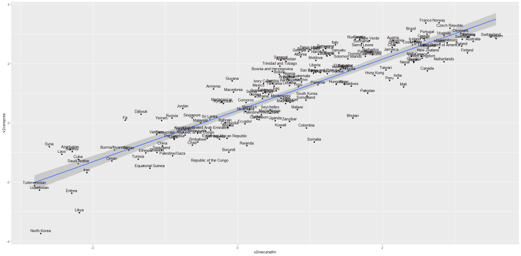
If we run a simple regression

summary(repression_model <- lm(media_censorship ~ civil_society_repression, data = data_2010))
stargazer(repression_model, type = "text")

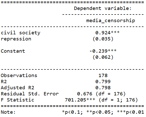
This is pretty common sense; a country that represses its citizens in one sphere is more likely to repress in other areas. In this case repressing the media correlates with repressing civil society.

We can plot the residuals of the above model with the autoplot() function from the ggfortify package.

library(ggfortify)
autoplot(repression_model)

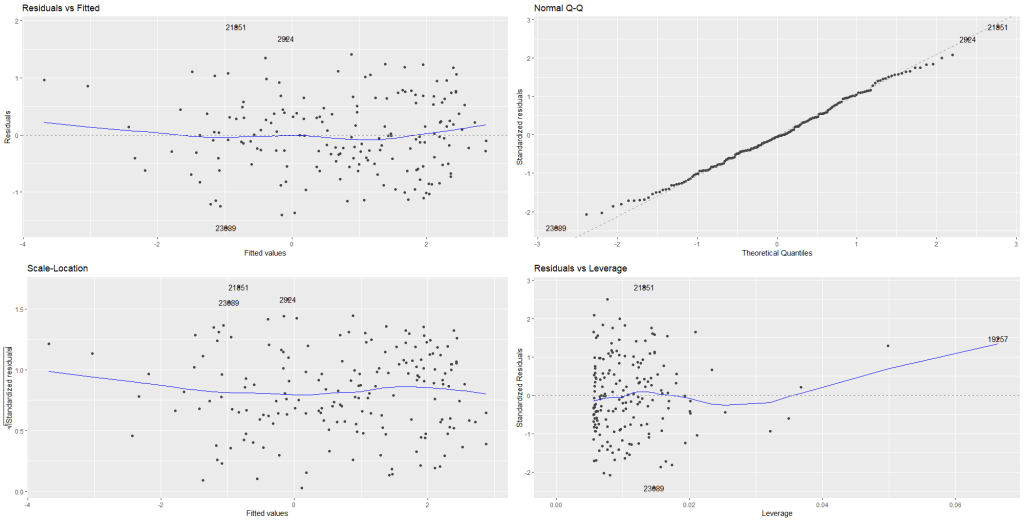
Nothing unusual appears to jump out at us with regard to evidence for heteroskedasticity!

In the first Residuals vs Fitted plot, we can see that blue line does not drastically diverge from the dotted line (which indicates residual value = 0).

The third plot Scale-Location shows again that there is no drastic instances of heteroskedasticity. We want to see the blue line relatively horizontal. There is no clear pattern in the distribution of the residual points.

In the Residual vs. Leverage plot (plot number 4), the high leverage observation 19257 is North Korea! A usual suspect when we examine model outliers.

While it is helpful to visually see the residuals plotted out, a more objective test can help us find whether the model is indeed free from heteroskedasticity problems.

For this we need the Breusch-Pagan test for heteroskedasticity from the lmtest package.

install.packages("lmtest)
library(lmtest)
bptest(repression_model)

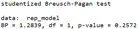
The default in R is the studentized Breusch-Pagan. However if you add the studentize = FALSE argument, you have the non-studentized version

The null hypothesis of the Breusch-Pagan test is that the variance in the model is homoskedastic.

With our repression_model, we cannot reject the null, so we can say with confidence that there is no major heteroskedasticity issue in our model.

The non-studentized Breusch-Pagan test makes a very big assumption that the error term is from Gaussian distribution. Since this assumption is usually hard to verify, the default bptest() in R “studentizes” the test statistic and provide asymptotically correct significance levels for distributions for error.

Why do we care about heteroskedasticity?

If our model demonstrates high level of heteroskedasticity (i.e. the random variables have non-random variation across observations), we run into problems.

Why?

  • OLS uses sub-optimal estimators based on incorrect assumptions and
  • The standard errors computed using these flawed least square estimators are more likely to be under-valued. Since standard errors are necessary to compute our t – statistics and arrive at our p – value, these inaccurate standard errors are a problem.

Example of heteroskedasticity

Let’s look at an example of this homoskedasticity assumption NOT being satisfied.

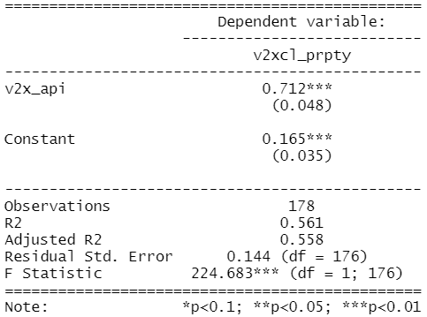
I run a simple regression to see whether there is a relationship between democracy score and respect for individuals’ private property rights in 178 countries in 2010.

When you are examining democracy as the main dependent variable, heteroskedasticity is a common complaint. This is because all highly democratic countries are all usually quite similar. However, when we look at autocracies, they are all quite different and seem to march to the beat of their own despotic drum. We cannot assume that the random variance across different regime types is equally likely.

First, let’s have a look at the relationship.

prop_graph <- ggplot(vdem2010, aes(v2xcl_prpty, v2x_api)) 
                     + geom_point(size = 3, aes(color = factor(regime_type))) 
                     + geom_smooth(method = "lm")
prop_graph + scale_colour_manual(values = c("#D55E00", "#E69F00", "#009E73", "#56B4E9"))

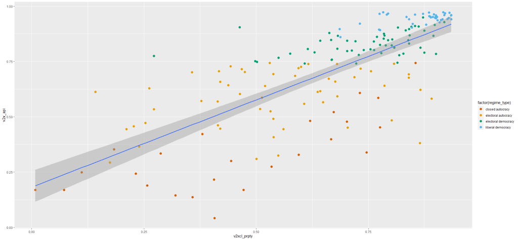
Next, let’s fit the model to examine the relationship.

summary(property_model <- lm(property_score ~ democracy_score, data = data_2010))
stargazer(property_model, type = "text")

To plot the residuals (and other diagnostic graphs) of the model, we can use the autoplot() function to look at the relationship in the model graphically.

autoplot(property_model)

Graph number 1 plots the residuals against the fitted model and we can see that lower values on the x – axis (fitted values) correspond with greater spread on the y – axis. Lower democracy scores relate to greater error on property rights index scores. Plus the blue line does not lie horizontal and near the dotted line. It appears we have non-random error patterns.

Examining the Scale – Location graph (number 3), we can see that the graph is not horizontal.

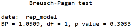
Again, interpreting the graph can be an imprecise art. So a more objective approach may be to run the bptest().

bptest(property_model)

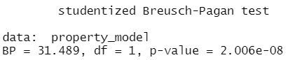
Since the p – value is far smaller than 0.05, we can reject the null of homoskedasticity.

Rather, we have evidence that our model suffers from heteroskedasticity. The standard errors in the regression appear smaller than they actually are in reality. This inflates our t – statistic and we cannot trust our p – value.

In the next blog post, we can look at ways to rectify this violation of homoskedasticity and to ensure that our regression output has more accurate standard errors and therefore more accurate p – values.

Click here to use the sandwich package to fix heteroskedasticity in the OLS regression.

Make Wes Anderson themed graphs with wesanderson package in R

Well this is just delightful! This package was created by Karthik Ram.

install.packages("wesanderson")
library(wesanderson)
library(hrbrthemes) # for plot themes
library(gapminder) # for data
library(ggbump) # for the bump plot

After you install the wesanderson package, you can

  1. create a ggplot2 graph object
  2. choose the Wes Anderson color scheme you want to use and create a palette object
  3. add the graph object and and the palette object and behold your beautiful data
Wes Anderson Trailer GIF - Find & Share on GIPHY
wes_palette(name, n, type = c("discrete", "continuous"))

To generate a vector of colors, the wes_palette() function requires:

  • name: Name of desired palette
  • n: Number of colors desired (i.e. how many categories so n = 4).

The names of all the palettes you can enter into the wes_anderson() function

Click here to look at more palette and theme packages that are inspired by Studio Ghibli, Dutch Master painters, Google, AirBnB, the Economist and Wall Street Journal aesthetics and appearances.

We can use data from the gapminder package. We will look at the scatterplot between life expectancy and GDP per capita.

We feed the wes_palette() function into the scale_color_manual() with the values = wes_palette() argument.

We indicate that the colours would be the different geographic regions.

If we indicate fill in the geom_point() arguments, we would change the last line to scale_fill_manual()

We can log the gapminder variables with the mutate(across(where(is.numeric), log)). Alternatively, we could scale the axes when we are at the ggplot section of the code with the scale_*_continuous(trans='log10')

gapminder %>% 
  filter(continent != "Oceania") %>% 
  mutate(across(where(is.numeric), log)) %>% 
  ggplot(aes(x = lifeExp, y = gdpPercap)) + 
  geom_point(aes(color = continent), size = 3, alpha = 0.8) +
  # facet_wrap(~factor(continent)) +
  hrbrthemes::theme_ft_rc() + 
  ggtitle("GDP per capita and life expectancy") + 
  theme(legend.title = element_blank(),
        legend.text = element_text(size = 20),
        plot.title = element_text(size = 30)) +
  scale_color_manual(values= wes_palette("FantasticFox1", n = 4)) +

Wes Anderson Trailer GIF - Find & Share on GIPHY

Next looking at bump plot of OECD data with the Royal Tenanbaum’s colour palette.

Click here to read more about the OECD dataset.

trust %>% 
  filter(country_name == "Ireland" | country_name == "Sweden" | country_name == "Germany" | country_name == "Spain" | country_name == "Belgium") %>% 
  group_by(year) %>%
  mutate(rank_budget = rank(-trust, ties.method = "min"),
         rank_budget = as.factor(rank_budget)) %>%
  ungroup()  %>% 
  ggplot(aes(x = year, y  = reorder(rank_budget, desc(rank_budget)), 
             group = country_name,
             color = country_name, fill = country_name)) +
  geom_bump(aes(), 
            smooth = 7,
            size = 5, alpha = 0.9) + 
  geom_point(aes(color = country_name), fill = "white", 
             shape = 21, size = 5, stroke = 5) +
  labs(title = "Level of trust in government",
       subtitle = "Data Source: OECD") + 
  theme(panel.border = element_blank(),
        legend.position = "bottom",
        plot.title = element_text(size = 30),
        legend.title = element_blank(),
        legend.text = element_text(size = 20, color = "white"),
        axis.text.y = element_text(size = 20), 
        axis.text.x = element_text(size = 20),
        legend.background = element_rect(fill = "#5e6472"),
        axis.title = element_blank(),
        axis.text = element_text(color = "white", size = 10),
        text= element_text(size = 15, color = "white"),
        panel.grid.major.y = element_blank(),
        panel.grid.minor.y = element_blank(),
        panel.grid.major.x = element_blank(),
        panel.grid.minor.x = element_blank(),
        legend.key = element_rect(fill = "#5e6472"),
        plot.background = element_rect(fill = "#5e6472"),
        panel.background = element_rect(fill = "#5e6472")) +
  guides(colour = guide_legend(override.aes = list(size=8))) +
  scale_color_manual(values= wes_palette("Royal2", n = 5)) +
  scale_x_continuous(n.breaks = 20)

Click here to read more about the bump plot from the ggbump package.

Last, we can look at Darjeeling colour palette.

trust %>% 
  filter(country_name == "Ireland" | country_name == "Germany" | country_name == "Sweden"| country_name == "Spain" | country_name == "Belgium") %>% 
  ggplot(aes(x = year,
             y = trust, group = country_name)) +
  geom_line(aes(color = country_name), size = 3) +
  geom_point(aes(color = country_name), fill = "white", shape = 21, size = 5, stroke = 5) +
  labs(title = "Level of trust in government",
       subtitle = "Data Source: OECD") + 
  theme(panel.border = element_blank(),
        legend.position = "bottom",
        plot.title = element_text(size = 30),
        legend.title = element_blank(),
        legend.text = element_text(size = 20, color = "white"),
        axis.text.y = element_text(size = 20), 
        axis.text.x = element_text(size = 20),
        legend.background = element_rect(fill = "#5e6472"),
        axis.title = element_blank(),
        axis.text = element_text(color = "white", size = 10),
        text= element_text(size = 15, color = "white"),
        panel.grid.major.y = element_blank(),
        panel.grid.minor.y = element_blank(),
        panel.grid.major.x = element_blank(),
        panel.grid.minor.x = element_blank(),
        legend.key = element_rect(fill = "#5e6472"),
        plot.background = element_rect(fill = "#5e6472"),
        panel.background = element_rect(fill = "#5e6472")) +
  guides(colour = guide_legend(override.aes = list(size=8))) +
  scale_color_manual(values= wes_palette("Darjeeling1", n = 5)) +
  scale_x_continuous(n.breaks = 20) 

Last we can look at a bar chart counting different regime types in the eighteenth century.

eighteenth_century <- data_1880s %>%
filter(!is.na(regime)) %>%
filter(!is.na(appointment)) %>%
ggplot(aes(appointment)) + geom_bar(aes(fill = factor(regime)), position = position_stack(reverse = TRUE)) + theme(legend.position = "top", text = element_text(size=15), axis.text.x = element_text(angle = -30, vjust = 1, hjust = 0))

Both the regime variable and the appointment variable are discrete categories so we can use the geom_bar() function. When adding the palette to the barplot object, we can use the scale_fill_manual() function.

eighteenth_century + scale_fill_manual(values = wes_palette("Darjeeling1", n = 4)

Now to compare the breakdown with countries in the 21st century (2000 to present)

Wes Anderson GIF - Find & Share on GIPHY

Add Correlates of War codes with countrycode package in R

One problem with merging two datasets by country is that the same countries can have different names. Take for example, America. It can be entered into a dataset as any of the following:

  • USA
  • U.S.A.
  • America
  • United States of America
  • United States
  • US
  • U.S.

This can create a big problem because datasets will merge incorrectly if they think that US and America are different countries.

Correlates of War (COW) is a project founded by Peter Singer, and catalogues of all inter-state war since 1963. This project uses a unique code for each country.

For example, America is 2.

When merging two datasets, there is a helpful R package that can convert the various names for a country into the COW code:

install.packages("countrycode")
library(countrycode)

To read more about the countrycode package in the CRAN PDF, click here.

First create a new name for the variable I want to make; I’ll call it COWcode in the dataset.

Then use the countrycode() function. First type in the brackets the name of the original variable that contains the list of countries in the dataset. Then finally add "country.name", "cown". This turns the word name for each country into the numeric COW code.

dataset$COWcode <- countrycode(dataset$countryname, "country.name", "cown")

If you want to turn into a country name, swap the "country.name" and "cown"

dataset$countryname <- countrycode(dataset$COWcode, "country.name", "cown")

Now the dataset is ready to merge more easily with my other dataset on the identical country variable type!

There are many other types of codes that you can add to your dataset.

A very popular one is the ISO-2 and ISO-3 codes. For example, if you want to add flags to your graph, you will need a two digit code for each country (for example, Ireland is IE).

To see the list of all the COW codes, click here.

To check out the COW database website, click here.

Alternative codes than the country.name and the cown options include:

• ccTLD: IANA country code top-level domain
• country.name: country name (English)
• country.name.de: country name (German)
• cowc: Correlates of War character
• cown: Correlates of War numeric
• dhs: Demographic and Health Surveys Program
• ecb: European Central Bank
• eurostat: Eurostat
• fao: Food and Agriculture Organization of the United Nations numerical code
• fips: FIPS 10-4 (Federal Information Processing Standard)
• gaul: Global Administrative Unit Layers
• genc2c: GENC 2-letter code
• genc3c: GENC 3-letter code
• genc3n: GENC numeric code
• gwc: Gleditsch & Ward character
• gwn: Gleditsch & Ward numeric
• imf: International Monetary Fund
• ioc: International Olympic Committee
• iso2c: ISO-2 character
• iso3c: ISO-3 character
• iso3n: ISO-3 numeric
• p4n: Polity IV numeric country code
• p4c: Polity IV character country code
• un: United Nations M49 numeric codes
4 codelist
• unicode.symbol: Region subtag (often displayed as emoji flag)
• unpd: United Nations Procurement Division
• vdem: Varieties of Democracy (V-Dem version 8, April 2018)
• wb: World Bank (very similar but not identical to iso3c)
• wvs: World Values Survey numeric code

# Some of my own manual COW code fixes
manual_cow_codes <- tibble::tribble(
  ~country,                 ~cow_code,
  "Palestinian Authority",   999,
  "Micronesia",              987,
  "Serbia"                   345
)