Replicating Eurostat graphs in R

Packages we will need:

library(eurostat)
library(tidyverse)
library(maggritr)
library(ggthemes)
library(forcats)

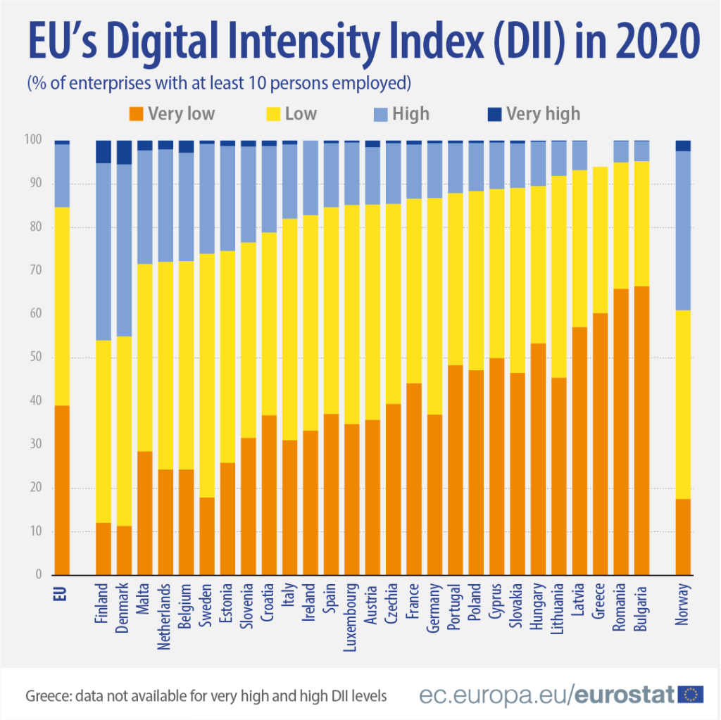
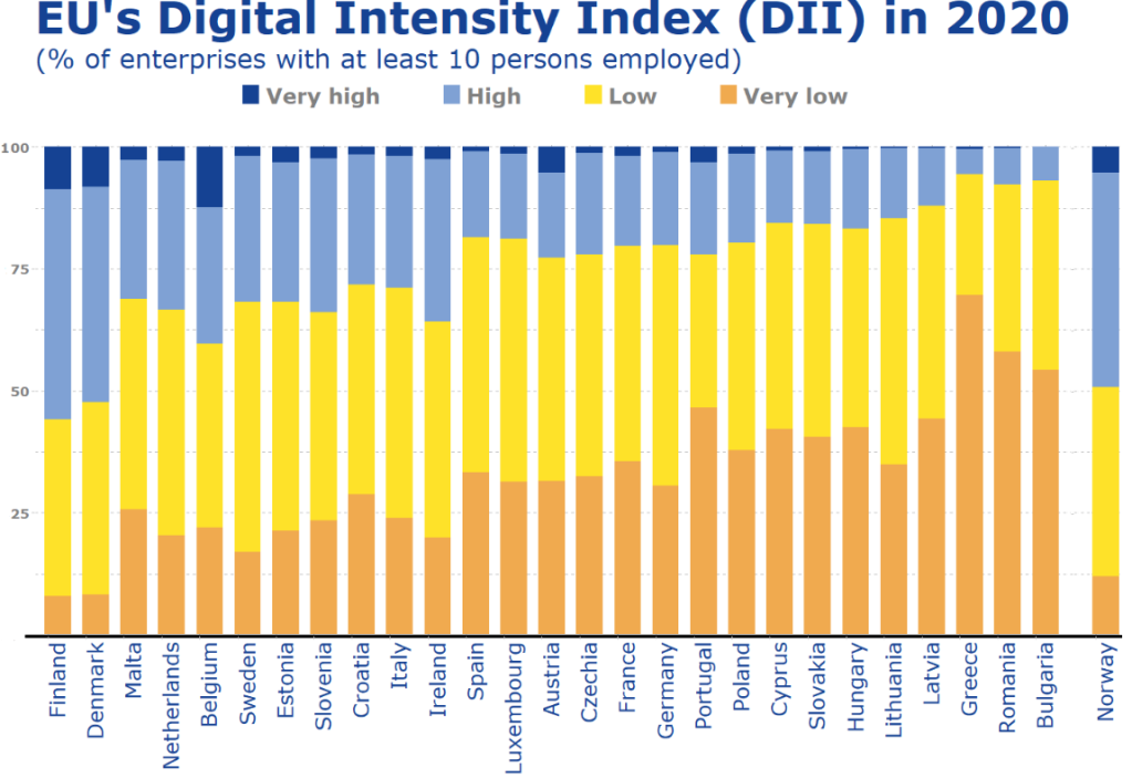
In this blog, we will try to replicate this graph from Eurostat!

It compares all European countries on their Digitical Intensity Index scores in 2020. This measures the use of different digital technologies by enterprises.

The higher the score, the higher the digital intensity of the enterprise, ranging from very low to very high.

For more information on the index, I took the above information from this site: https://ec.europa.eu/eurostat/web/products-eurostat-news/-/ddn-20211029-1

First, we will download the digital index from Eurostat with the get_eurostat() function.

Click here to learn more about downloading data on EU from the Eurostat package.

Next some data cleaning. To copy the graph, we will aggregate the different levels into very low, low, high and very high categories with the grepl() function in some ifelse() statements.

The variable names look a bit odd with lots of blank space because I wanted to space out the legend in the graph to replicate the Eurostat graph above.

dig <- get_eurostat("isoc_e_dii", type = "label")

dig %<>% 
   mutate(dii_level = ifelse(grepl("very low", indic_is), "Very low        " , ifelse(grepl("with low", indic_is), "Low        ", ifelse(grepl("with high", indic_is), "High        ", ifelse(grepl("very high", indic_is), "Very high        ", indic_is)))))

Next I fliter out the year I want and aggregate all industry groups (from the sizen_r2 variable) in each country to calculate a single DII score for each country.

dig %>% 
  select(sizen_r2, geo, values, dii_level, year) %>%  
  filter(year == 2020) %>% 
  group_by(dii_level, geo) %>% 
  summarise(total_values = sum(values, na.rm = TRUE)) %>% 
  ungroup() -> my_dig

I use a hex finder website imagecolorpicker.com to find the same hex colors from the Eurostat graph and assign them to our version.

dii_pal <- c("Very low        " = "#f0aa4f",
             "Low        " = "#fee229",
             "Very high        " = "#154293", 
             "High        " = "#7fa1d4")

We can make sure the factors are in the very low to very high order (rather than alphabetically) with the ordered() function

my_dig$dii_level <- ordered(my_dig$dii_level, levels = c("Very Low        ", "Low        ", "High        ","Very high        "))

Next we filter out the geo rows we don’t want to add to the the graph.

Also we can change the name of Germany to remove its longer title.

my_dig %>% 
  filter(geo != "Euro area (EA11-1999, EA12-2001, EA13-2007, EA15-2008, EA16-2009, EA17-2011, EA18-2014, EA19-2015)") %>% 
  filter(geo != "United Kingdom") %>% 
  filter(geo != "European Union - 27 countries (from 2020)") %>% 
  filter(geo != "European Union - 28 countries (2013-2020)") %>% 
  mutate(geo = ifelse(geo == "Germany (until 1990 former territory of the FRG)", "Germany", geo)) -> my_dig

And also, to have the same order of countries that are in the graph, we can add them as ordered factors.

my_dig$country <- factor(my_dig$geo, levels = c("Finland", "Denmark", "Malta", "Netherlands", "Belgium", "Sweden", "Estonia", "Slovenia", "Croatia", "Italy", "Ireland","Spain", "Luxembourg", "Austria", "Czechia", "France", "Germany", "Portugal", "Poland", "Cyprus", "Slovakia", "Hungary", "Lithuania", "Latvia", "Greece", "Romania", "Bulgaria", "Norway"), ordered = FALSE)

Now to plot the graph:

my_dig %>% 
  filter(!is.na(country)) %>% 
  group_by(country, dii_level) %>% 
  ggplot(aes(y = country, 
             x = total_values,
             fill = forcats::fct_rev(dii_level))) +
  geom_col(position = "fill", width = 0.7) + 
  scale_fill_manual(values = dii_pal) + 
  ggthemes::theme_pander() +
  coord_flip() +
  labs(title = "EU's Digital Intensity Index (DII) in 2020",
       subtitle = ("(% of enterprises with at least 10 persons employed)"),
       caption = "ec.europa/eurostat") +
  xlab("") + 
  ylab("") + 
  theme(text = element_text(family = "Verdana", color = "#154293"),
        axis.line.x = element_line(color = "black", size = 1.5),
        axis.text.x = element_text(angle = 90, size = 20, color = "#154293", hjust = 1),
        axis.text.y = element_text(color = "#808080", size = 13, face = "bold"),
        legend.position = "top", 
        legend.title = element_blank(),
        legend.text = element_text(color = "#808080", size = 20, face = "bold"),
        plot.title = element_text(size = 42, color = "#154293"),
        plot.subtitle = element_text(size = 25, color = "#154293"),
        plot.caption = element_text(size = 20, color = "#154293"),
        panel.background = element_rect(color = "#f2f2f2"))

It is not identical and I had to move the black line up and the Norway model more to the right with Paint on my computer! So a bit of cheating!

Click to read Part 1, Part 2 and Part 3 of the blog series on visualising Eurostat data

For information on the index discussed in this blog post: https://ec.europa.eu/eurostat/web/products-eurostat-news/-/ddn-20211029-1

Visualize EU data with Eurostat package in R: Part 2 (with maps)

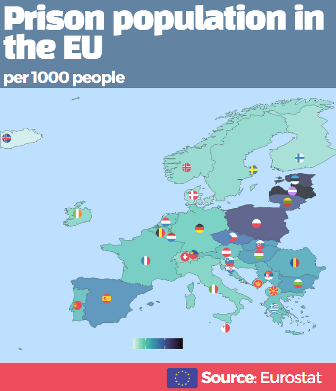
In this post, we will map prison populations as a percentage of total populations in Europe with Eurostat data.

library(eurostat)
library(tidyverse)
library(sf)
library(rnaturalearth)
library(ggthemes)
library(countrycode)
library(ggflags)
library(viridis)
library(rvest)

Click here to read Part 1 about downloading Eurostat data.


prison_pop <- get_eurostat("crim_pris_pop", type = "label")

prison_pop$iso3 <- countrycode::countrycode(prison_pop$geo, "country.name", "iso3c")

prison_pop$year <- as.numeric(format(prison_pop$time, format = "%Y"))

Next we will download map data with the rnaturalearth package. Click here to read more about using this package.

We only want to zoom in on continental EU (and not include islands and territories that EU countries have around the world) so I use the coordinates for a cropped European map from this R-Bloggers post.

map <- rnaturalearth::ne_countries(scale = "medium", returnclass = "sf")

europe_map <- sf::st_crop(map, xmin = -20, xmax = 45,
                          ymin = 30, ymax = 73)

prison_map <- merge(prison_pop, europe_map, by.x = "iso3", by.y = "adm0_a3", all.x = TRUE)

We will look at data from 2000.

prison_map %>% 
  filter(year == 2000) -> map_2000

To add flags to our map, we will need ISO codes in lower case and longitude / latitude.

prison_map$iso2c <- tolower(countrycode(prison_map$geo, "country.name", "iso2c"))

coord <- read_html("https://developers.google.com/public-data/docs/canonical/countries_csv")

coord_tables <- coord %>% html_table(header = TRUE, fill = TRUE)

coord <- coord_tables[[1]]

prison_map <- merge(prison_map, coord, by.x= "iso_a2", by.y = "country", all.y = TRUE)

Nex we will plot it out!

We will focus only on European countries and we will change the variable from total prison populations to prison pop as a percentage of total population. Finally we multiply by 1000 to change the variable to per 1000 people and not have the figures come out with many demical places.

prison_map %>% 
  filter(continent == "Europe") %>% 
  mutate(prison_pc = (values / pop_est)*1000) %>% 
  ggplot() +
  geom_sf(aes(fill = prison_pc, geometry = geometry), 
          position = "identity") + 
  labs(fill='Prison population')  +
  ggflags::geom_flag(aes(x = longitude, 
                         y = latitude+0.5, 
                         country = iso2_lower), 
                     size = 9) +  
  scale_fill_viridis_c(option = "mako", direction = -1) +
  ggthemes::theme_map() -> prison_map

Next we change how it looks, including changing the background of the map to a light blue colour and the legend.

prison_map + 
  theme(legend.title = element_text(size = 20),
        legend.text = element_text(size = 14), 
         legend.position = "bottom",
        legend.background = element_rect(fill = "lightblue",
                                         colour = "lightblue"),
        panel.background = element_rect(fill = "lightblue",
                                        colour = "lightblue"))

I will admit that I did not create the full map in ggplot. I added the final titles and block colours with canva.com because it was just easier! I always find fonts very tricky in R so it is nice to have dozens of different fonts in Canva and I can play around with colours and font sizes without needing to reload the plot each time.

Add circular flags to maps and graphs with ggflags package in R

Packages we will need:

library(ggflags)
library(bbplot) # for pretty BBC style graphs
library(countrycode) # for ISO2 country codes
library(rvest) # for webscrapping

Click here to add rectangular flags to graphs and click here to add rectangular flags to MAPS!

Always Sunny Charlie GIF by It's Always Sunny in Philadelphia - Find & Share on GIPHY

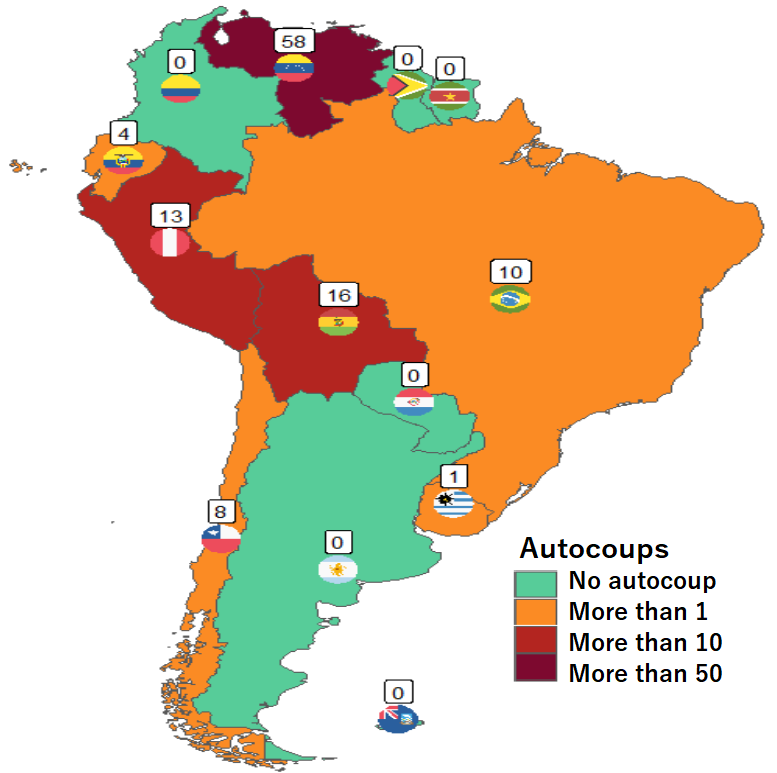
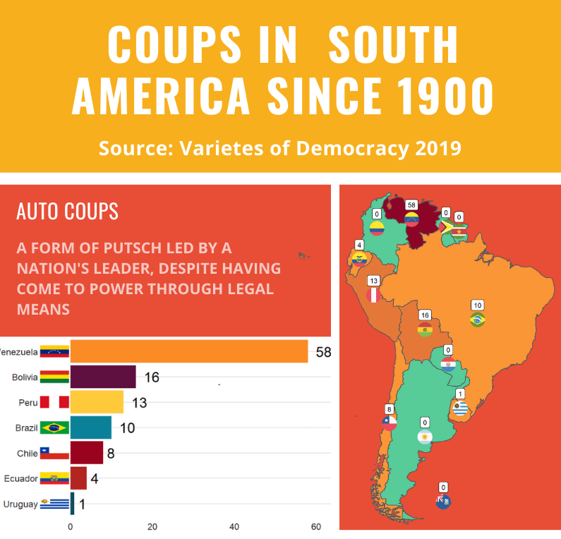
Apropos of this week’s US news, we are going to graph the number of different or autocoups in South America and display that as both maps and bar charts.

According to our pals at the Wikipedia, a self-coup, or autocoup (from the Spanish autogolpe), is a form of putsch or coup d’état in which a nation’s leader, despite having come to power through legal means, dissolves or renders powerless the national legislature and unlawfully assumes extraordinary powers not granted under normal circumstances.

In order to add flags to maps, we need to make sure our dataset has three variables for each country:

Charlie Day Cat GIF by Maudit - Find & Share on GIPHY

Longitude
Latitude
ISO2 code (in lower case)

In order to add longitude and latitude, I will scrape these from a website with the rvest dataset and merge them with my existing dataset.

Click here to learn more about the rvest pacakge.

library(rvest)

coord <- read_html("https://developers.google.com/public-data/docs/canonical/countries_csv")

coord_tables <- coord %>% html_table(header = TRUE, fill = TRUE)

coord <- coord_tables[[1]]

map_df2 <- merge(map_df, coord, by.x= "iso_a2", by.y = "country", all.y = TRUE)

Click here to learn more about the merge() function

Next we need to add a variable with each country’s ISO code with the countrycode() function

Click here to learn more about the countrycode package.

autocoup_df$iso2c <- countrycode(autocoup_df$country_name, "country.name", "iso2c")

In this case, a warning message pops up to tell me:

Some values were not matched unambiguously: Kosovo, Somaliland, Zanzibar

One important step is to convert the ISO codes from upper case to lower case. The geom_flag() function from the ggflag package only recognises lower case (e.g Chile is cl, not CL).

autocoup_df$iso2_lower <- tolower(autocoup_df$iso_a2)

We have all the variables we will need for our geom_flag() function:

Add some hex colors as a vector that we can add to the graph:

coup_palette  <- c("#7d092f", "#b32520", "#fb8b24", "#57cc99")

Finally we can graph our maps comparing the different types of coups in South America.

Click here to learn how to graph variables onto maps with the rnaturalearth package.

The geom_flag() function requires an x = longitude, y = latitude and a country argument in the form of our lower case ISO2 country codes. You can play around the latitude and longitude flag and also label position by adding or subtracting from them. The size of the flag can be added outside the aes() argument.

We can place the number of coups under the flag with the geom_label() function.

The theme_map() function we add comes from ggthemes package.

autocoup_map <- autocoup_df%>% 
  dplyr::filter(subregion == "South America") %>%
  ggplot() +
  geom_sf(aes(fill = coup_cat)) +
  ggflags::geom_flag(aes(x = longitude, y = latitude+0.5, country = iso2_lower), size = 8) +
  geom_label(aes(x = longitude, y = latitude+3, label = auto_coup_sum, color = auto_coup_sum), fill  =  "white", colour = "black") +
  theme_map()
 
 
autocoup_map + scale_fill_manual(values = coup_palette, name = "Auto Coups", labels = c("No autocoup", "More than 1", "More than 10", "More than 50"))

Not hard at all.

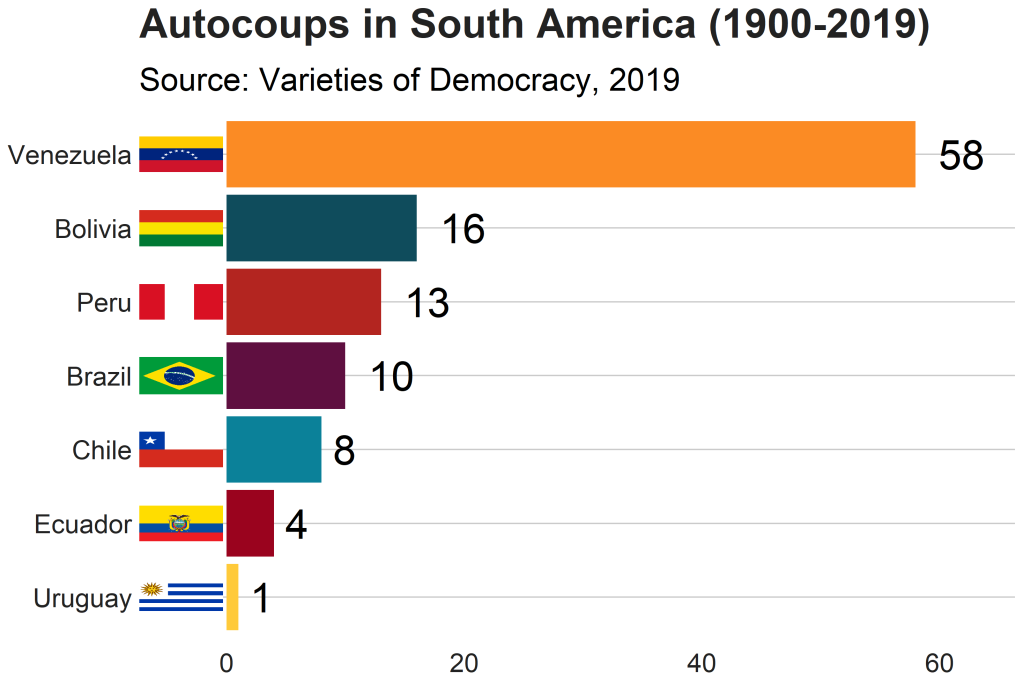
And we can make a quick barchart to rank the countries. For this I will use square flags from the ggimage package. Click here to read more about the ggimage package

Additionally, I will use the theme from the bbplot pacakge. Click here to read more about the bbplot package.

library(ggimage)
library(bbplot)

pretty_colors <- c("#0f4c5c", "#5f0f40","#0b8199","#9a031e","#b32520","#ffca3a", "#fb8b24")

autocoup_df %>% 
  dplyr::filter(auto_coup_sum !=0) %>% 
  dplyr::filter(subregion == "South America") %>%
  ggplot(aes(x = reorder(country_name, auto_coup_sum), 
             y = auto_coup_sum, 
             group = country_name, 
             fill = country_name)) +
  geom_col() +
  coord_flip() +
  bbplot::bbc_style() +
  geom_text(aes(label = auto_coup_sum), 
            hjust = -0.5, size = 10,
            position = position_dodge(width = 1),
            inherit.aes = TRUE) +
  expand_limits(y = 63) +
  labs(title = "Autocoups in South America (1900-2019)",
       subtitle = "Source: Varieties of Democracy, 2019") +
  theme(legend.position = "none") +
  scale_fill_manual(values = pretty_colors) +
  ggimage::geom_flag(aes(y = -4, 
                         image = iso2_lower), 
                         size = 0.1)

And after a bit of playing around with all three different types of coup data, I created an infographic with canva.com

Add Correlates of War codes with countrycode package in R

One problem with merging two datasets by country is that the same countries can have different names. Take for example, America. It can be entered into a dataset as any of the following:

USA
U.S.A.
America
United States of America
United States
US
U.S.

This can create a big problem because datasets will merge incorrectly if they think that US and America are different countries.

Correlates of War (COW) is a project founded by Peter Singer, and catalogues of all inter-state war since 1963. This project uses a unique code for each country.

For example, America is 2.

When merging two datasets, there is a helpful R package that can convert the various names for a country into the COW code:

install.packages("countrycode")
library(countrycode)

To read more about the countrycode package in the CRAN PDF, click here.

First create a new name for the variable I want to make; I’ll call it COWcode in the dataset.

Then use the countrycode() function. First type in the brackets the name of the original variable that contains the list of countries in the dataset. Then finally add "country.name", "cown". This turns the word name for each country into the numeric COW code.

dataset$COWcode <- countrycode(dataset$countryname, "country.name", "cown")

If you want to turn into a country name, swap the "country.name" and "cown"

dataset$countryname <- countrycode(dataset$COWcode, "country.name", "cown")

Now the dataset is ready to merge more easily with my other dataset on the identical country variable type!

There are many other types of codes that you can add to your dataset.

A very popular one is the ISO-2 and ISO-3 codes. For example, if you want to add flags to your graph, you will need a two digit code for each country (for example, Ireland is IE).

To see the list of all the COW codes, click here.

To check out the COW database website, click here.

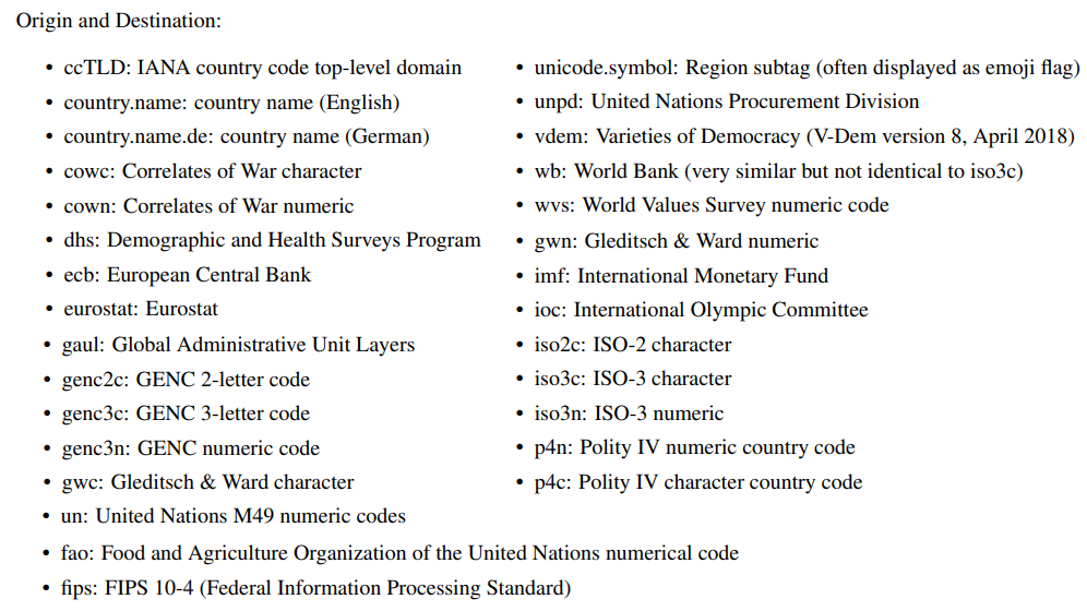
Alternative codes than the country.name and the cown options include:

• ccTLD: IANA country code top-level domain
• country.name: country name (English)
• country.name.de: country name (German)
• cowc: Correlates of War character
• cown: Correlates of War numeric
• dhs: Demographic and Health Surveys Program
• ecb: European Central Bank
• eurostat: Eurostat
• fao: Food and Agriculture Organization of the United Nations numerical code
• fips: FIPS 10-4 (Federal Information Processing Standard)
• gaul: Global Administrative Unit Layers
• genc2c: GENC 2-letter code
• genc3c: GENC 3-letter code
• genc3n: GENC numeric code
• gwc: Gleditsch & Ward character
• gwn: Gleditsch & Ward numeric
• imf: International Monetary Fund
• ioc: International Olympic Committee
• iso2c: ISO-2 character
• iso3c: ISO-3 character
• iso3n: ISO-3 numeric
• p4n: Polity IV numeric country code
• p4c: Polity IV character country code
• un: United Nations M49 numeric codes
4 codelist
• unicode.symbol: Region subtag (often displayed as emoji flag)
• unpd: United Nations Procurement Division
• vdem: Varieties of Democracy (V-Dem version 8, April 2018)
• wb: World Bank (very similar but not identical to iso3c)
• wvs: World Values Survey numeric code