How to graph bubble charts and treemap charts in R

Packages we will need:

library(tidyverse)
library(bubbles)
library(treemapify)
library(democracyData)
library(magrittr)

In this blog, we will look at different types of charts that we can run in R.

Approve Always Sunny GIF by It's Always Sunny in Philadelphia - Find & Share on GIPHY

Both the bubble and treemap charts are simple to run.

Before we begin, we will choose some hex colors for the palette. I always use the coolors palettes website to find nice colours.

pal <- c("#bc4749", "#005f73", 
         "#0a9396", "#94d2bd", 
         "#bb3e03","#003049",
         "#fca311", "#99d98c",
         "#9a5059", "#ee9b00")

First, we can download the data we will graph.

In this case, we will use the DD (democracies and dictatorships) regime data from PACL dataset on different government regimes.

The DD dataset encompasses annual data points for 199 countries spanning from 1946 to 2008. The visual representations on the left illustrate the outcomes in 1988 and 2008.

Cheibub, Gandhi, and Vreeland devised a six-fold regime classification scheme, giving rise to what they termed the DD datasets. The DD index categorises regimes into two types: democracies and dictatorships.

Democracies are divided into three types: parliamentary, semi-presidential, and presidential democracies.

Dictatorships are subcategorized into monarchic, military, and civilian dictatorship.

democracyData::pacl -> pacl

First, we create a new variable with the regime names, not just the number. The values come from the codebook.

Tv Show Drinking GIF - Find & Share on GIPHY
pacl %<>% 
  mutate(regime_name = ifelse(regime == 0, "Parliamentary democracies",
                 ifelse(regime == 1, "Mixed democracies",
                 ifelse(regime == 2, "Presidential democracies",
                 ifelse(regime == 3, "Civilian autocracies",
                 ifelse(regime == 4, "Military dictatorships",
                 ifelse(regime ==  5,"Royal dictatorships", regime))))))) %>%
  mutate(regime = as.factor(regime)) 
  order pacl_country  year regime_name        
  <dbl> <chr>        <dbl> <chr>              
1     1 Afghanistan   1946 Royal dictatorships
2     2 Afghanistan   1947 Royal dictatorships
3     3 Afghanistan   1948 Royal dictatorships
4     4 Afghanistan   1949 Royal dictatorships
5     5 Afghanistan   1950 Royal dictatorships
6     6 Afghanistan   1951 Royal dictatorships

We want to count the number of different regime types.

pacl %>% 
  group_by(regime_name) %>% 
  count() -> pacl_count

We can graph out the geom_treemap() layer in the ggplot() object

pacl_count %>% 
  ggplot(aes(area = n, fill = regime_name, 
           label = paste(regime_name, n, sep = "\n"))) +
  geom_treemap(color = "white", size = 3) +
  geom_treemap_text(
    place = "centre",
    size = 20) +
  theme(legend.position = "none") + 
  scale_fill_manual(values = sample(pal)) 

And we can use the bubbles() function from the bubbles package.

Unfortunately, it is not pipable into ggplot, so it is hard to edit factors such as the font size.

bubbles::bubbles(label = pacl_count$regime_name,
                 value = pacl_count$n, 
                 color = sample(pal, size = length(pacl_count$regime_name)))

Thank you for reading!

Top R packages for downloading political science and economics datasets

  1. WDI
  2. peacesciencer
  3. eurostat
  4. vdem
  5. democracyData
  6. icpsrdata
  7. Quandl
  8. essurvey
  9. manifestoR
  10. unvotes
  11. gravity

1. WDI

The World Development Indicators (WDI) package by Vincent Arel-Bundock provides access to a database of hundreds of economic development indicators from the World Bank.

Examples of variables include population, GDP, education, health, and poverty, school attendance rates.

Reference: Arel-Bundock, V. (2017). WDI: World Development Indicators (R Package Version 2.7.1).

2. peacesciencer

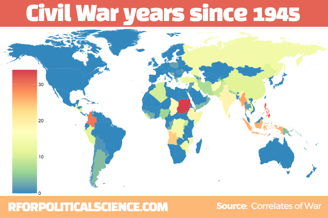
This package by Steve Miller helps you download data related to peace and conflict studies, including the Correlates of War project.

Examples of variables include Alliance Treaty Obligations and Provisions (ATOP), Thompson and Dreyer’s (2012) strategic rivalry data, fractionalization/polarization estimates from the Composition of Religious and Ethnic Groups (CREG) Project, and Uppsala Conflict Data Program (UCDP) data on civil and inter-state conflicts.

Data can come in either country-year, event-level or dyadic-level.

Reference: Steve Miller (2020). peacesciencer: Tools for Peace Scientists (R Package Version 0.2.2). Website retrieved at http://svmiller.com/peacesciencer/ms.html

3. eurostat

eurostat provides access to a wide range of statistics and data on the European Union and its member states, covering topics such as population, economics, society, and the environment.

Examples of variables include employment, inflation, education, crime, and air pollution. The package was authored by Leo Lahti.

Reference: eurostat (2018). eurostat: Eurostat Open Data (R Package Version 3.6.0), CRAN PDF retrieved at https://cran.r-project.org/web/packages/eurostat/eurostat.pdf

4. vdemdata

The Varieties of Democracy package by Staffan I. Lindberg et al. provides data on a range of indicators related to democracy and governance in countries around the world, including measures of electoral democracy, civil liberties, and human rights.

Click here to read more about downloading the package

Examples of variables include freedom of speech, rule of law, corruption, government transparency, and voter turnout.

Reference: Lindberg, S. I., & Stepanova, N. (2020). vdem: Varieties of Democracy Project (R Package Version 1.6).

5. democracyData

This package by Xavier Marquez: provides data on a range of variables related to democracy, including elections, political parties, and civil liberties.

Examples of variables include regime type, democracy scores (Freedom House, PolityIV etc,  Geddes, Wright, and Frantz’ autocratic regimes dataset, the Lexical Index of Electoral Democracy, the DD/ACLP/PACL/CGV dataset), axxording to the Github page

6. icpsrdata

This package by Frederick Solt provides a simple way to download and import data from the Inter-university Consortium for Political and Social Research (ICPSR) archive into R. This is for easy replication and sharing of data. The package includes datasets from different fields of study, including sociology, political science, and economics.

Reference: Solt, F. (2020). icpsrdata: Reproducible Data Retrieval from the ICPSR Archive (R Package Version 0.5.0).

7. Quandl

This R package by Quandl provides an interface to access financial and economic data from over 20 different sources. Examples of variables include stock prices, futures, options, and macroeconomic indicators. The package includes functions to easily download data directly into R and perform tasks such as plotting, transforming, and aggregating data. Additional functions for managing and exploring data, such as search tools and data caching features, are also available.

Here are five examples of variables in the Quandl package:

  • “AAPL” (Apple Inc. stock price)
  • “CHRIS/CME_CL1” (Crude Oil Futures)
  • “FRED/GDP” (US GDP)
  • “BCHAIN/MKPRU” (Bitcoin Market Price)
  • “USTREASURY/YIELD” (US Treasury Yield Curve Rates)

Reference: Quandl. (2021). Quandl: A library of economic and financial data. Retrieved from https://www.quandl.com/tools/r.

8. essurvey

The essurvey package is an R package that provides access to data from the European Social Survey (ESS), which is a large-scale survey that collects data on attitudes, values, and behavior across Europe. The package includes functions to easily download, read, and analyze data from the ESS, and also includes documentation and sample code to help users get started.

Examples of variables in the ESS dataset include political interest, trust in political institutions, social class, education level, and income. The package was authored by David Winter and includes a variety of useful functions for working with ESS data.

Reference: Winter, D. (2021). essurvey: Download Data from the European Social Survey on the Fly. R package version 3.4.4. Retrieved from https://cran.r-project.org/package=essurvey.

9. manifestoR

manifestoR is an R package that provides access to data from the Comparative Manifesto Project (CMP), which is a cross-national research project that analyzes political party manifestos. The package allows users to easily download and analyze data from the CMP, including party positions on various policy issues and the salience of those issues across time and space.

Examples of variables in the CMP dataset include party positions on taxation, immigration, the environment, healthcare, and education. The package was authored by Jörg Matthes, Marcelo Jenny, and Carsten Schwemmer.

Reference: Matthes, J., Jenny, M., & Schwemmer, C. (2018). manifestoR: Access and Process Data and Documents of the Manifesto Project. R package version 1.2.1. Retrieved from https://cran.r-project.org/package=manifestoR.

10. unvotes

The unvotes data package provides historical voting data of the United Nations General Assembly, including votes for each country in each roll call, as well as descriptions and topic classifications for each vote.

The classifications included in the dataset cover a wide range of issues, including human rights, disarmament, decolonization, and Middle East-related issues.

Reference: The package was created by David Robinson and Nicholas Goguen-Compagnoni and is available on the Comprehensive R Archive Network (CRAN) at https://cran.r-project.org/web/packages/unvotes/unvotes.pdf.

11. gravity

The gravity package in R, created by Anna-Lena Woelwer, provides a set of functions for estimating gravity models, which are used to analyze bilateral trade flows between countries. The package includes the gravity_data dataset, which contains information on trade flows between pairs of countries.

Examples of variables that may affect trade in the dataset are GDP, distance, and the presence of regional trade agreements, contiguity, common official language, and common currency.

iso_o: ISO-Code of country of origin
iso_d: ISO-Code of country of destination
distw: weighted distance
gdp_o: GDP of country of origin
gdp_d: GDP of country of destination
rta: regional trade agreement
flow: trade flow
contig: contiguity
comlang_off: common official language
comcur: common currency

The package PDF CRAN is available at http://cran.nexr.com/web/packages/gravity/gravity.pdf

Cleaning up messy World Bank data

Packages we will need:

library(tidyverse)
library(tidyr)
library(janitor)
library(magrittr)
library(democracyData)
library(countrycode)
library(ggimage)

When you come across data from the World Bank, often it is messy.

So this blog will go through how to make it more tidy and more manageable in R

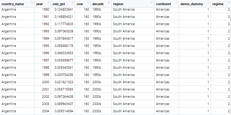
For this blog, we will look at World Bank data on financial aid. Specifically, we will be using values for net ODA received as percentage of each country’s GNI. These figures come from the Development Assistance Committee of the Organisation for Economic Co-operation and Development (DAC OECD).

If we look at the World Bank data downloaded from the website, we have a column for each year and the names are quite messy.

This data is wide form.

Unacceptable.

So we will change the data from wide to long data.

Instead of a column for each year, we will have a row for each country-year.

Before doing that, we can clean up the variable names with the janitor package function: clean_names().

sdg %<>% 
  clean_names() 

ALSO, before we pivot the dataset to longer format, we choose the variables we want to keep (i.e. only country, year and ODA value)

sdg %<>% 
  select(country_name, x1990_yr1990:x2015_yr2015) 

Now we are ready to turn the data from wide to long.

We can use the pivot_longer() function from the tidyr package.

Instead of 286 rows and 27 columns, we will ultimately end up with 6968 rows and only 3 columns.

Source: Garrick Aden-Buie’s (@grrrckTidy Animated Verbs

Thank you to Mr. Aden-Buie for your page visualising all the different ways to transform datasets with dplyr. Click the link to check out more.

Back to the pivoting, we want to create a row for each year, 1990, 1991, 1992 …. up to 2015

And we will have a separate cell for each value of the ODA variable for each country-year value.

In the pivot_longer() function we exclude the country names,

We want a new row for each year, so we make a “year” variable with the names_to() argument.

And we create a separate value for each ODA as a percentage of GNI with the values_to() argument.

sdg %>% 
  pivot_longer(!country_name, names_to = "year", 
               values_to = "oda_gni") -> oda

The year values are character strings, not numbers. So we will convert with parse_number(). This parses the first number it finds, dropping any non-numeric characters before the first number and all characters after the first number.

oda %>% 
     mutate(year = parse_number(year)) -> oda 

Next we will move from the year variable to ODA variable. There are many ODA values that are empty. We can see that there are 145 instances of empty character strings.

oda %>% 
  count(oda_gni) %>% 
  arrange(oda_gni)

So we can replace the empty character strings with NA values using the na_if() function. Then we can use the parse_number() function to turn the character into a string.

oda %>%
  mutate(oda_gni = na_if(oda_gni, "")) %>% 
  mutate(oda_gni = parse_number(oda_gni)) -> oda

Now we need to delete the year variables that have no values.

oda %<>% 
  filter(!is.na(year))

Also we need to delete non-countries.

The dataset has lots of values for regions that are not actual countries. If you only want to look at politically sovereign countries, we can filter out countries that do not have a Correlates of War value.

oda %<>%
  mutate(cow = countrycode(oda$country_name, "country.name", 'cown')) %>% 
  filter(!is.na(cow))

We can also make a variable for each decade (1990s, 2000s etc).

oda %>% 
  mutate(decade = substr(year, 1, 3)) %>% 
  mutate(decade = paste0(decade, "0s"))

And download data for countries’ region, continent and govenment regime. To do this we use the democracyData package and download the PACL dataset.

Click here to read more about this package.

pacl <- democracyData::redownload_pacl()

pacl %>% 
  select(cow = pacl_cowcode,
         year,
         region = un_region_name,
         continent = un_continent_name,
         demo_dummy = democracy,
         regime = regime
         ) -> pacl_subset

We use the left_join() function to join both datasets together with Correlates of War code and year variables.

oda %>% 
  left_join(pacl_subset, by = c("cow", "year")) -> oda_pacl

Now if we look at the dataset, we can see that it is much tidier and we can start analysing.

Below we can create a bar chart of the top ten countries that received the most aid as a percentage of their economic income (gross national income)

First we need to get the average oda per country with the group_by() and summarise() functions

oda_pacl %>%
  mutate(oda_gni = ifelse(is.na(oda_gni), 0, oda_gni)) %>%  
  group_by(country_name,region, continent) %>% 
  summarise(avg_oda = mean(oda_gni, na.rm = TRUE)) -> oda_mean

We use the slice() function to only have the top ten countries

oda_mean %>% 
  arrange(desc(avg_oda)) %>%
  ungroup() %>% 
  slice(1:10) -> oda_slice

We add an ISO code for each country for the flags

Click here to read more about the ggimage package

oda_slice %<>% 
  mutate(iso2 = countrycode(country_name, "country.name", "iso2c"))

And some nice hex colours

my_palette <- c( "#44bec7", "#ffc300", "#fa3c4c")

And finally, plot it out with ggplot()

oda_slice %>%
  ggplot(aes(x = reorder(country_name, avg_oda),
             y = avg_oda, fill = continent)) + 
  geom_bar(stat = "identity") + 
  ggimage::geom_flag(aes(image = iso2), size = 0.1)  +
  coord_flip() +
  scale_fill_manual(values = my_palette) + 
  labs(title = "ODA aid as % GNI ",
       subtitle = "Source: OECD DAC via World Bank",
       x = "Donor Country",
       y = "ODA per capita") + bbplot::bbc_style()

Scraping and wrangling UN peacekeeping data with tidyr package in R

Packages we will need:

library(tidyverse)
library(rvest)
library(magrittr)
library(tidyr)
library(countrycode)
library(democracyData)
library(janitor)
library(waffle)

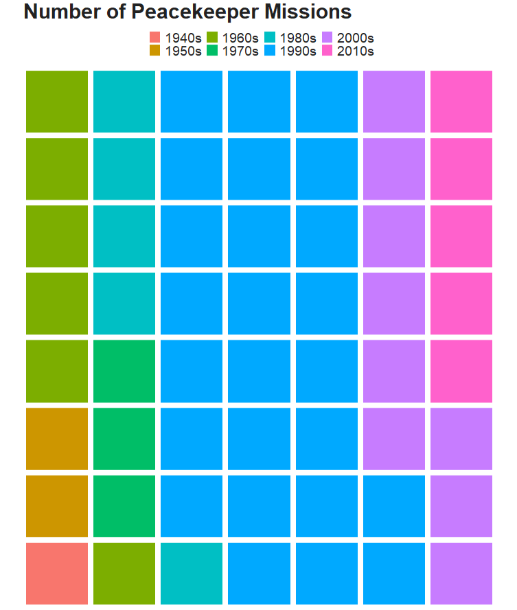
For this blog post, we will look at UN peacekeeping missions and compare across regions.

Despite the criticisms about some operations, the empirical record for UN peacekeeping records has been robust in the academic literature

“In short, peacekeeping intervenes in the most difficult
cases, dramatically increases the chances that peace will
last, and does so by altering the incentives of the peacekept,
by alleviating their fear and mistrust of each other, by
preventing and controlling accidents and misbehavior by
hard-line factions, and by encouraging political inclusion”
(Goldstone, 2008: 178).

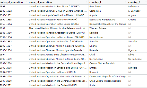
The data on the current and previous PKOs (peacekeeping operations) will come from the Wikipedia page. But the variables do not really lend themselves to analysis as they are.

Amy Coney Barrett Snl GIF by Saturday Night Live - Find & Share on GIPHY

Once we have the url, we scrape all the tables on the Wikipedia page in a few lines

pko_members <- read_html("https://en.wikipedia.org/wiki/List_of_United_Nations_peacekeeping_missions")
pko_tables <- pko_members %>% html_table(header = TRUE, fill = TRUE)

Click here to read more about the rvest package for scraping data from websites.

pko_complete_africa <- pko_tables[[1]]
pko_complete_americas <- pko_tables[[2]]
pko_complete_asia <- pko_tables[[3]]
pko_complete_europe <- pko_tables[[4]]
pko_complete_mena <- pko_tables[[5]]

And then we bind them together! It’s very handy that they all have the same variable names in each table.

rbind(pko_complete_africa, pko_complete_americas, pko_complete_asia, pko_complete_europe, pko_complete_mena) -> pko_complete

Next, we will add a variable to indicate that all the tables of these missions are completed.

pko_complete %<>% 
  mutate(complete = ifelse(!is.na(pko_complete$Location), "Complete", "Current"))

We do the same with the current missions that are ongoing:

pko_current_africa <- pko_tables[[6]]
pko_current_asia <- pko_tables[[7]]
pko_current_europe <- pko_tables[[8]]
pko_current_mena <- pko_tables[[9]]

rbind(pko_current_europe, pko_current_mena, pko_current_asia, pko_current_africa) -> pko_current

pko_current %<>% 
  mutate(complete = ifelse(!is.na(pko_current$Location), "Current", "Complete"))

We then bind the completed and current mission data.frames

rbind(pko_complete, pko_current) -> pko

Then we clean the variable names with the function from the janitor package.

pko_df <-  pko %>% 
  janitor::clean_names()

Next we’ll want to create some new variables.

We can make a new row for each country that is receiving a peacekeeping mission. We can paste all the countries together and then use the separate function from the tidyr package to create new variables.

 pko_df %>%
  group_by(conflict) %>%
  mutate(location = paste(location, collapse = ', ')) %>% 
  separate(location,  into = c("country_1", "country_2", "country_3", "country_4", "country_5"), sep = ", ")  %>% 
  ungroup() %>% 
  distinct(conflict, .keep_all = TRUE) %>% 

Next we can create a new variable that only keeps the acroynm for the operation name. I took these regex codes from the following stack overflow link

pko_df %<>% 
  mutate(acronym = str_extract_all(name_of_operation, "\\([^()]+\\)")) %>% 
  mutate(acronym = substring(acronym, 2, nchar(acronym)-1)) %>% 
  separate(dates_of_operation, c("start_date", "end_date"), "–")

I will fill in the end data for the current missions that are still ongoing in 2022

pko_df %<>% 
  mutate(end_date = ifelse(complete == "Current", 2022, end_date)) 

And next we can calculate the duration for each operation

pko_df %<>% 
  mutate(end_date = as.integer(end_date)) %>% 
  mutate(start_date = as.integer(start_date)) %>% 
  mutate(duration = ifelse(!is.na(end_date), end_date - start_date, 1)) 

I want to compare regions and graph out the different operations around the world.

We can download region data with democracyData package (best package ever!)

Snl Season 47 GIF by Saturday Night Live - Find & Share on GIPHY
pacl <- redownload_pacl()

pacl %>% 
  select(cown = pacl_cowcode,
        un_region_name, un_continent_name) %>% 
  distinct(cown, .keep_all = TRUE) -> pacl_region

We join the datasets together with the inner_join() and add Correlates of War country codes.

pko_df %<>% 
  mutate(cown = countrycode(country_1, "country.name", "cown")) %>%   mutate(cown = ifelse(country_1 == "Western Sahara", 605, 
                       ifelse(country_1 == "Serbia", 345, cown))) %>% 
  inner_join(pacl_region, by = "cown")

Now we can start graphing our duration data:

pko_df %>% 
  ggplot(mapping = aes(x = forcats::fct_reorder(un_region_name, duration), 
                       y = duration, 
                       fill = un_region_name)) +
  geom_boxplot(alpha = 0.4) +
  geom_jitter(aes(color = un_region_name),
              size = 6, alpha = 0.8, width = 0.15) +
  coord_flip() + 
  bbplot::bbc_style() + ggtitle("Duration of Peacekeeping Missions")
Years

We can see that Asian and “Western Asian” – i.e. Middle East – countries have the longest peacekeeping missions in terns of years.

pko_countries %>% 
  filter(un_continent_name == "Asia") %>%
  unite("country_names", country_1:country_5, remove = TRUE,  na.rm = TRUE, sep = ", ") %>% 
  arrange(desc(duration)) %>% 
  knitr::kable("html")
Start End Duration Region Country
1949 2022 73 Southern Asia India, Pakistan
1964 2022 58 Western Asia Cyprus, Northern Cyprus
1974 2022 48 Western Asia Israel, Syria, Lebanon
1978 2022 44 Western Asia Lebanon
1993 2009 16 Western Asia Georgia
1991 2003 12 Western Asia Iraq, Kuwait
1994 2000 6 Central Asia Tajikistan
2006 2012 6 South-Eastern Asia East Timor
1988 1991 3 Southern Asia Iran, Iraq
1988 1990 2 Southern Asia Afghanistan, Pakistan
1965 1966 1 Southern Asia Pakistan, India
1991 1992 1 South-Eastern Asia Cambodia, Cambodia
1999 NA 1 South-Eastern Asia East Timor, Indonesia, East Timor, Indonesia, East Timor
1958 NA 1 Western Asia Lebanon
1963 1964 1 Western Asia North Yemen
2012 NA 1 Western Asia Syria

Next we can compare the decades

pko_countries %<>% 
  mutate(decade = substr(start_date, 1, 3)) %>% 
  mutate(decade = paste0(decade, "0s")) 

And graph it out:

pko_countries %>% 
  ggplot(mapping = aes(x = decade, 
                       y = duration, 
                       fill = decade)) +
  geom_boxplot(alpha = 0.4) +
  geom_jitter(aes(color = decade),
              size = 6, alpha = 0.8, width = 0.15) +
   coord_flip() + 
  geom_curve(aes(x = "1950s", y = 60, xend = "1940s", yend = 72),
  arrow = arrow(length = unit(0.1, "inch")), size = 0.8, color = "black",
   curvature = -0.4) +
  annotate("text", label = "First Mission to Kashmir",
           x = "1950s", y = 49, size = 8, color = "black") +
  geom_curve(aes(x = "1990s", y = 46, xend = "1990s", yend = 32),
             arrow = arrow(length = unit(0.1, "inch")), size = 0.8, color = "black",curvature = 0.3) +
  annotate("text", label = "Most Missions after the Cold War",
           x = "1990s", y = 60, size = 8, color = "black") +

  bbplot::bbc_style() + ggtitle("Duration of Peacekeeping Missions")
Years

Following the end of the Cold War, there were renewed calls for the UN to become the agency for achieving world peace, and the agency’s peacekeeping dramatically increased, authorizing more missions between 1991 and 1994 than in the previous 45 years combined.

We can use a waffle plot to see which decade had the most operation missions. Waffle plots are often seen as more clear than pie charts.

Click here to read more about waffle charts in R

To get the data ready for a waffle chart, we just need to count the number of peacekeeping missions (i.e. the number of rows) in each decade. Then we fill the groups (i.e. decade) and enter the n variable we created as the value.

pko_countries %>% 
  group_by(decade) %>% 
  count() %>%  
  ggplot(aes(fill = decade, values = n)) + 
  waffle::geom_waffle(color = "white", size= 3, n_rows = 8) +
  scale_x_discrete(expand=c(0,0)) +
  scale_y_discrete(expand=c(0,0)) +
  coord_equal() +
  labs(title = "Number of Peacekeeper Missions") + bbplot::bbc_style() 
Cecily Strong Snl GIF by Saturday Night Live - Find & Share on GIPHY

If we want to add more information, we can go to the UN Peacekeeping website and download more data on peacekeeping troops and operations.

We can graph the number of peacekeepers per country

Click here to learn more about adding flags to graphs!

le_palette <- c("#5f0f40", "#9a031e", "#94d2bd", "#e36414", "#0f4c5c")

pkt %>%
  mutate(contributing_country = ifelse(contributing_country == "United Republic of Tanzania", "Tanzania",ifelse(contributing_country == "Côte d’Ivoire", "Cote d'Ivoire", contributing_country))) %>% 
  mutate(iso2 = tolower(countrycode::countrycode(contributing_country, "country.name", "iso2c"))) %>% 
  mutate(cown = countrycode::countrycode(contributing_country, "country.name", "cown")) %>% 
  inner_join(pacl_region, by = "cown") %>% 
  mutate(un_region_name = case_when(grepl("Africa", un_region_name) ~ "Africa",grepl("Eastern Asia", un_region_name) ~ "South-East Asia",
 un_region_name == "Western Africa" ~ "Middle East",TRUE ~ as.character(un_region_name))) %>% 
  filter(total_uniformed_personnel > 700) %>% 
  ggplot(aes(x = reorder(contributing_country, total_uniformed_personnel),
             y = total_uniformed_personnel)) + 
  geom_bar(stat = "identity", width = 0.7, aes(fill = un_region_name), color = "white") +
  coord_flip() +
  ggflags::geom_flag(aes(x = contributing_country, y = -1, country = iso2), size = 8) +
  # geom_text(aes(label= values), position = position_dodge(width = 0.9), hjust = -0.5, size = 5, color = "#000500") + 
  scale_fill_manual(values = le_palette) +
  labs(title = "Total troops serving as peacekeepers",
       subtitle = ("Across countries"),
       caption = "         Source: UN ") +
  xlab("") + 
  ylab("") + bbplot::bbc_style()

We can see that Bangladesh, Nepal and India have the most peacekeeper troops!